The sign says average waiting time: twenty minutes. Somewhere near the wall, one person has begun to recognise the pattern in the upholstery. The sign can be correct. So can that person’s sense that the afternoon is disappearing.

THE EVERYDAY SYSTEMS LABORATORYNO. 008 / OPERATIONS & PROBABILITY

The Shape of Waiting.

AN INTERACTIVE QUEUE-DISTRIBUTION LABORATORY

The average has excellent manners.
The queue has other ideas.

Change a rule. Follow a person. Read the whole distribution.

Opening the counters. The laboratory loads as you approach.

Published 21 October 2026 · Updated 21 October 2026

Begin with the person at the edge

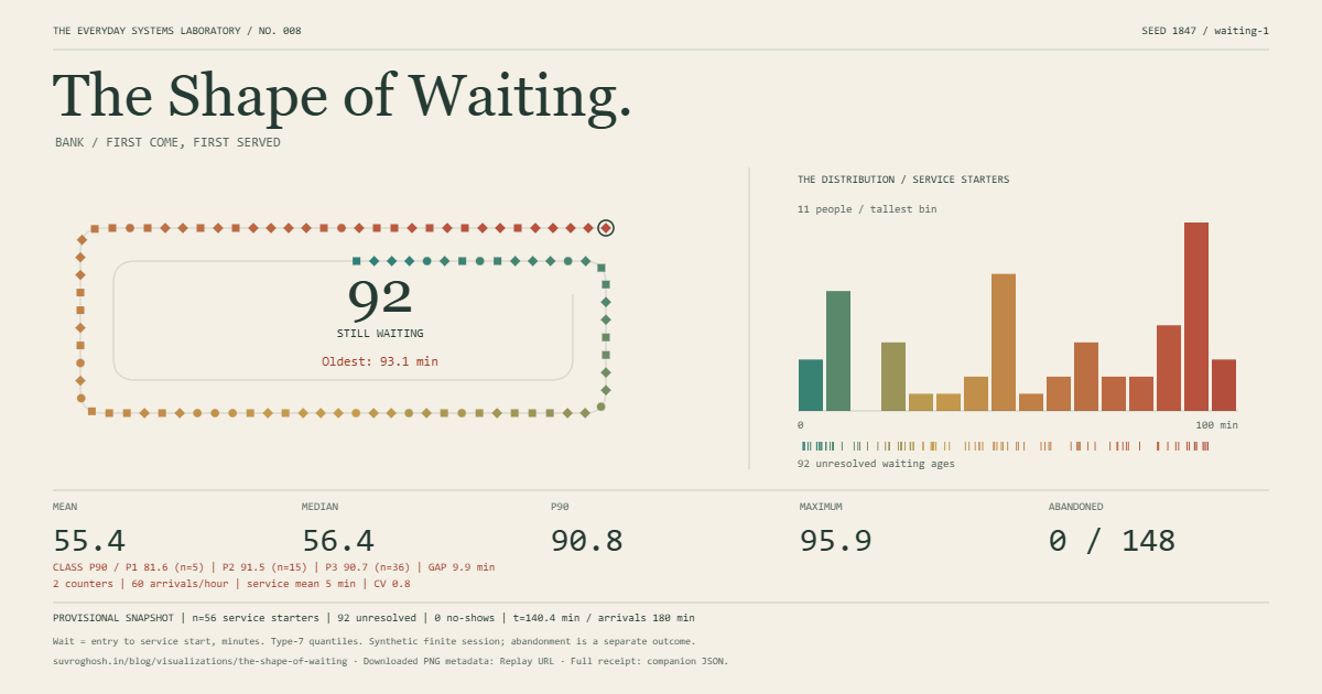
Each ticket belongs to one synthetic person, caller or message. It joins the line, waits, and either starts service or leaves. Position follows the scheduling order. Colour records waiting age on the same scale across the laboratory, so a red ticket cannot become reassuringly teal merely because the rest of the queue grew older.

Choose Follow the oldest. The inspector gives that ticket a history: when it arrived, its class, whether later arrivals entered service first, and how long it has waited. A mark on a distribution has acquired an address.

The stage is an operational picture. The histogram is its accounting. Finished waits collect into a distribution with mean, median and 90th percentile marked. The separate strip of current waiting ages shows people whose final wait is still unknown. Watch both before deciding that the system has improved.

Three experiments, the same arrivals

Start with One more counter. Keep the original run as a baseline and add capacity. The paired view reuses the same arrivals and underlying demands. You can select the same ticket in both versions of the day.

Next try Same mean, more uncertainty. The configured expected service duration stays fixed while the spread changes. A few lengthy jobs can occupy counters while shorter jobs accumulate behind them. In a finite sample, the realised average service duration can fluctuate even though its generating distribution has the same expected value.

Finally choose Better average, worse tail. This is a reproducible worked example, with the affected tail measure identified in the comparison. Read the class rows as well as the headline. A policy can favour many tickets while concentrating delay among fewer tickets. A lower mean answers one question. It leaves several others open.

Changing the seed asks the model another version of the question. These are paired synthetic experiments; one attractive screenshot cannot establish a universal effect.

Seven waiting rooms

The bank pools ordinary arrivals across counters. The railway counter receives concentrated bursts. The visa office groups work into batches, with formation delays and setup costs. The clinic admits scheduled appointments and records no-shows separately. The call centre allows finite patience. The emergency department gives synthetic urgency classes non-preemptive priority: service already in progress finishes before another ticket can take that counter. The business inbox turns people into messages with uneven amounts of work.

Each preset changes its operational assumptions. None is calibrated to a real institution. A patient and an unanswered email may share queue mathematics while carrying very different human consequences.

Open the advanced controls to change the rule. First come, first served respects arrival order. Random selection can leave an early arrival behind; its displayed queue ranking is illustrative because the next selection redraws the order. Priority favours the configured class; ageing lets time already spent waiting increase a ticket’s claim on the next available server. These choices have visible consequences for who gets overtaken.

Batching has a formation rule, a maximum delay and a capacity cost. A no-show never joins the queue. Abandonment happens after joining it. Keeping those outcomes distinct prevents a system from looking efficient simply because its visitors disappeared.

Whose average is this?

The primary waiting-time sample contains tickets whose service has started. Their wait is service-start time minus queue-entry time. It does not include service duration. The interface names this population and its count; during playback, its summaries are provisional.

Someone still waiting has a current age, but no observed final waiting time. If observation ends now, that eventual time lies beyond what we have seen. This is the same lower-bound idea that underlies right-censored observations in the NIST statistical handbook. The laboratory displays current ages separately. It does not estimate a survival curve or quietly treat unfinished waits as zero.

Abandoned tickets have a different observed outcome: time until leaving. Their count, denominator and waiting-time summary remain separate from successfully started service. A caller who hangs up has not been answered.

The median describes the middle of the served-wait sample. P90 locates its upper region according to the stated sample-quantile convention. Maximum observed wait keeps even a tiny extreme visible. A small sample is labelled as such, and an empty sample receives an em dash rather than a fabricated zero.

For a final result, arrivals stop at the configured end of the session and the system drains. Existing service finishes. If a computation bound interrupts that process, the result explicitly retains its unresolved population and stopping time. These are finite-session experiments beginning from an empty system, rather than steady-state estimates.

Fair by which rule?

The class rows show median and p90 waits for the people each class actually served. Their gap makes a policy’s distributional effect inspectable. The overtaking measure asks how many service starters saw at least one later arrival begin service first.

Those measures answer different questions. Arrival-order adherence, equal class waits and urgency-based priority express different objectives. The laboratory makes no demographic assignments and produces no universal fairness score. Its synthetic classes let you inspect the cost of a chosen operational rule.

Try following the same ticket across a comparison. Then inspect the ticket that benefited. The trade-off becomes harder to hide inside a single number.

The clock inside the picture

The engine advances between discrete events: an arrival, a service completion, a patience deadline or an applicable batch event. A priority queue orders their simulated times, with explicit precedence and a stable tie-breaker. The SimPy scheduling documentation explains why events that share a displayed time still need deterministic ordering. This implementation uses its own TypeScript engine and publishes its particular tie rules in the model notes.

Animation time is separate. Playing faster changes how quickly the picture unfolds on your screen; it does not make a counter more efficient. Resizing, pausing or choosing Still leaves the model’s result intact.

The same frozen snapshot supplies the stage, summaries, inspector and export. The drawing cannot invent a more photogenic queue than the accounting supports. At large populations, the view can aggregate marks, with the count labelled and the oldest waiting ticket retained; the model still accounts for every ticket.

Take a waiting receipt

Download the PNG receipt for a compact view of the result, or the versioned JSON for the configuration and its numerical record. Both carry the seed, observation time, completion status, sample definitions and replay URL. The link opens the same bounded model and reruns it locally.

The receipt can make a claim precise: this rule, these arrivals, this population, this outcome. It cannot turn a classroom simulation into evidence about a real clinic, railway or office.

Return to the sign. Twenty minutes may still be a correct average. Now you know to look for the person it leaves outside the sentence.