A dataset can lose a third of its values in several very different ways. One looks like dust on a photographic plate. Another looks as though somebody has torn away the evening. Both can receive the same reassuring description: 67 per cent complete.
The Music of
Missing Data.
A dataset can lose a third of its values in several very different ways.
Change what disappears. Watch the silence take shape.
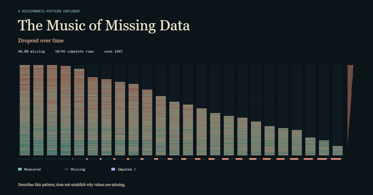
A matrix of light. A score of silences. The interactive instrument loads as you approach.
Published · Updated
Checking article narration…
Begin with the lights on
The matrix is a small, wholly synthetic world. In the multivariate view, a row is an observation and a column is a variable. In the longitudinal view, rows are participants and columns are successive visits for one measure. These are different questions, with different axes.
Colour records a value on a fixed scale. Darkness records its absence. A real zero remains a measured value; a hole never secretly becomes zero. Select a cell, or use the keyboard inspector, to read its identity and status.
Keep the seed and matrix view fixed while changing the disappearance rule. The complete data stay put. The instrument changes what would have been recorded, allowing a fair comparison. Reveal what vanished temporarily opens the envelope that a real analyst would never receive. The imputation methods cannot open it.
Seven ways to leave a silence
Start with Missing completely at random. Each eligible cell faces an independent draw that ignores its value and the other measurements. Holes scatter across the field. This is MCAR: the missingness process has no preference for the numbers it removes.
Next try Missing depending on observed information. A predictor remains fully observed, and its value changes the chance that another measurement disappears. This illustrates MAR. After conditioning on the observed predictor, the missingness rule has no remaining dependence on the unseen outcome.
With Missing depending on the missing value itself, the value about to vanish influences its own disappearance. The visible remainder can be systematically different from the complete sample. This is MNAR in the simulation: knowing the observed predictor still leaves a dependence on the hidden value.
The other presets describe collection processes. Dropout over time removes every visit after a participant leaves. Sort by dropout time and a diagonal shore emerges. Return to the original order and the same gaps look different. The calculations remain identical.
Entire missing variables takes out whole columns. Failed instruments creates temporary outages with recovery. Selective nonresponse removes responses preferentially from a defined part of the sample. Each preset names its actual simulated mechanism; a process name alone cannot establish MCAR, MAR or MNAR.
The National Research Council distinguishes these patterns from the assumptions about their causes. A visible diagonal can describe dropout without telling us why people left. The explorer knows the rule because it wrote it. The photograph of a real gap does not contain that privilege.
Same percentage. Different damage
Open Compare patterns. It holds the complete data and analysis target fixed while contrasting MCAR with a structured disappearance rule. Both request the same target percentage. Read the achieved rates: the rules can produce different counts, and whole columns restrict the percentages that can be attained.
The small summaries expose what an overall percentage compresses. A column may have lost nearly everything while its neighbours are intact. Many rows may share one missingness pattern. A pair of variables may repeatedly disappear together. Complete-case analysis then keeps only rows with every required measurement, sometimes discarding most of the sample.
The estimate panel supplies denominators as well as means. The available-data mean describes the measurements that remain. The complete synthetic-sample mean is a reference for this experiment. Their difference is estimation error in one sample. Calling that difference “bias” would require an appropriate repeated-sampling investigation.
Try seed 1847, the variables view, target 35 per cent, strength 2 and Measure 01. Switch between MCAR and MNAR without changing those settings. Both remove exactly 528 of 1,536 cells: 34.375 per cent. The selected column tells a different story:
| Measure 01 | Complete sample | MCAR remainder | MNAR remainder |
|---|---|---|---|
| Mean, score points | 49.948 | 50.650 | 45.811 |
| Measurements | 96 | 79 | 74 |
| Estimation error, points | — | +0.702 | −4.138 |
The same overall missing percentage conceals different denominators and errors. This is one reproducible synthetic sample, with no promise that the next seed behaves identically.
The embalmed dataset
Choose Column mean. The holes acquire values. Within each variable, every filled cell receives the same number. A busy surface becomes suspiciously orderly: small bands of preserved average, as though the dataset has been prepared for display.
The mean of that completed column equals the available-data mean, when a mean exists. That equality offers no guarantee that either equals the complete-sample mean. Repeated mean values also reduce variation. The apparent restoration has not restored the relationships the missing observations might have carried.
Every filled cell retains its imputation mark. For this method the inspector says uncertainty not estimated. A clean surface is no evidence that the uncertainty has gone away.
A wholly missing variable presents an even firmer boundary. There is no observed column mean, and no observed outcome on which to fit its conditional model. The explorer leaves it unfilled and says it is not estimable from these data.
Give the uncertainty somewhere to live
Switch to Conditional predictive draw. The model fits each variable using its observed values and the fully observed predictor. It then makes a reproducible draw for each missing cell. Choose another draw to see a different completion supported by those assumptions.
The halos represent the conditional model’s predictive spread, as defined in the inspector. They do not measure every possible error, establish the missingness mechanism or account for an unknown model being wrong. A narrow halo can accompany a bad assumption.
These are predictive draws. Proper multiple-imputation inference also analyses the completed datasets and combines the results with appropriate uncertainty accounting. The official mice documentation describes that broader workflow. This small instrument does not claim to perform it.
In the MNAR preset, move Missing-outcome sensitivity. The observed values remain fixed; assumptions about the missing outcomes shift. Watch the completed estimate move. The National Research Council’s sensitivity-analysis chapter explains why conclusions should be examined under departures from the assumptions used for the main analysis. Here the control is an educational, bounded version of that question: how much does our answer owe to what we supplied?
Listen to what is absent
Enable sound explicitly, then start the scan. The playhead follows the displayed rows, sounding at most eight evenly sampled columns per row. Columns retain fixed pentatonic pitches; values change their loudness on the same fixed score scale as the colours. Missing cells create rests. A legitimate zero can still sound.
If you enable audition of imputations, their different timbre announces their provenance. The mapping and volume do not secretly compensate for the missing observations. A sparser dataset can become a sparser phrase.
Sound is an additional way to notice structure. It cannot diagnose a mechanism, and the entire experiment works silently. Still mode keeps the explanatory marks stable; the prose, numerical summaries and cell inspector carry the same meaning without a travelling light.
Take the holes with you
Download the missingness fingerprint. The PNG arranges the current matrix, marginal summaries, settings and legend as a plate. Its companion JSON records the versioned seed, parameters, counts, ordering and imputation assumptions. The share link reopens a bounded simulation state.
The fingerprint describes this pattern; it does not establish why values are missing. Its usefulness lies in making a conversation specific. Which variables vanished together? Which estimate uses which rows? What did the filling procedure assume? Can somebody else reproduce the experiment?
Turn the lights back on once more. Then let the same numbers disappear another way. The silence has acquired a shape. The shape still needs a history.
Quick reference and FAQ
A missing value is a gap with a history. This explorer keeps a synthetic dataset fixed while changing which measurements disappear. Light and optional sound reveal the gaps; estimates and clearly marked imputations show what the gaps can change.
Key Terms
- Missingness pattern
- MCAR
- MAR
- MNAR
- Dropout
- Imputation
- Predictive draw
- Sensitivity analysis
- Complete case
Frequently asked questions
Can the picture tell me whether data are missing at random?
No. A pattern shows where values are absent. The explorer knows the mechanism because it generated the missingness. In real data, the observed mask alone cannot establish MCAR, MAR or MNAR.
Does a filled cell become an observed measurement?
No. An imputed cell permanently retains a separate marker. Mean filling estimates no uncertainty here; conditional predictive draws show model-dependent predictive spread. Neither recovers a measurement that was never observed.
Are the predictive draws multiple imputation?
This explorer shows alternative completions from a fitted conditional model. It does not pool repeated analyses using multiple-imputation inference, so it labels the completions predictive draws.
Can the explorer fill an entirely missing variable?
Its observed-data models cannot estimate a variable with no observations. Those cells remain missing and the inspector reports that the variable is not estimable from these data.
Do I need sound or WebGL to understand the article?
No. Sound starts only after an explicit action. Controls, textual summaries and a fallback matrix support silent exploration, and the poster and article remain readable without JavaScript.
Word Cloud
Related reading
Selected by shared topics and section, with closer publication dates breaking ties.