The Strange Attractor Orchestra: When Chaos Learns to Sing
Poster & listening mode
A curve enters weather—and sings.
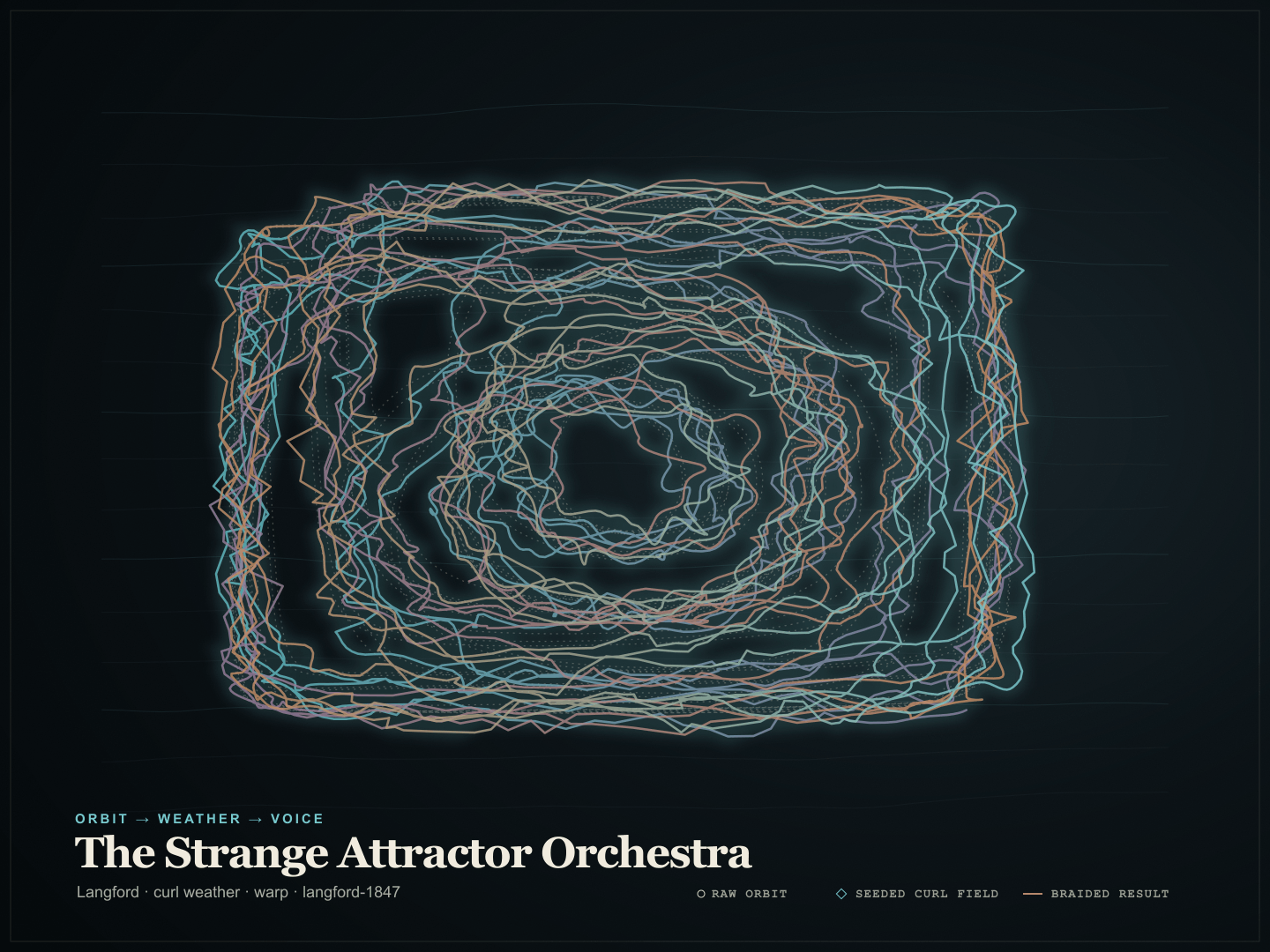
The canonical orbit remains intact. A seeded curl field bends only its visible copy; measured returns, regions and folds become a deterministic score.
Inspecting this screen before loading the instrument.
Preparing the wider conducting instrument. No WebGL point cloud, bloom, wake system or live diagnostic is loaded here.
Published · Updated
What am I looking at? A deterministic orbit is calculated at a fixed numerical step. A seeded field then bends or colours only the orbit’s visible copy. Crossings, folds, returns, density and the sampled field become one symbolic score, so a flash and a tone can share the same cause.
Uses the speech voice supplied by your browser or device.
Chaos is not dice
A strange attractor is not a line somebody drew while feeling cosmic. It is a region of phase space approached by a deterministic dynamical system: a compact record of the states that the system continues to visit after its transient behaviour has been discarded. The familiar Lorenz shape, for example, is not a butterfly icon hiding inside an equation. It is a projection of a three-variable trajectory whose nearby initial conditions may separate quickly even though the rule of motion contains no dice.
That distinction matters because unpredictability has several causes. A coin toss is difficult partly because its initial conditions are not measured well enough; radioactive decay is treated probabilistically at a more fundamental level; a pseudorandom generator is an algorithm producing a repeatable sequence; and a chaotic differential equation is deterministic yet sensitive. Put them all in a cupboard labelled random and the cupboard soon becomes useless.
The instrument begins with a registered equation, a registered parameter set, a registered initial condition and a fixed integration step. Continuous systems use fourth-order Runge–Kutta integration. The Hénon system is a discrete map and is therefore iterated directly. Mackey–Glass is a delay equation: its derivative depends on an interpolated value from its own history, so the displayed three-coordinate curve is a delay embedding, not a claim that the system literally possesses only three state variables.
Every preset is warmed before the page measures it. The warm-up is thrown away before the display bounds, recurrence grid or musical features are computed. After that, the observation coordinates are frozen with a robust transform. For coordinate ,
This makes very different systems fit inside one instrument without repeatedly squeezing the picture to whatever happened in the latest frame. It does not alter the canonical state. A non-finite value or a preset-specific escape-radius violation stops the calculation visibly; it is never wrapped, clamped or bullied back into the frame. A pretty clamped failure would be a different dynamical system wearing the first one’s name badge.
During validation, selected continuous presets are also compared at the registered step and at . Chaotic trajectories should not be expected to agree point by point after enough simulated time; sensitive dependence makes that a foolish test. The useful comparisons are robust bounds, occupancy, section crossings, return intervals and time-averaged diagnostics. The question is whether both computations describe the same statistical object at the scale claimed, not whether their millionth points have remained politely adjacent.
The Lorenz source is Edward Lorenz’s 1963 paper, “Deterministic Nonperiodic Flow”. Its exact divergence at the displayed parameters is . That contraction is a useful regression check. It is not, by itself, proof of chaos.
The curve enters weather
The raw orbit is the Orbit. The added field is the Weather. The music is the Voice. Keeping those nouns separate prevents the page from committing a common piece of graphical fraud: showing a deformed curve and quietly pretending that the deformation came from the differential equation.
Here the canonical trajectory is calculated first. A second, independently seeded layer samples coherent graphics noise at the frozen observation coordinates. Nearby locations receive related values, so the field has broad fronts and ridges rather than television static. Its phase advances in simulation time, not wall-clock time; a dropped visual frame can reduce detail but cannot move the scientific system to a different score.
Four kinds of weather are curated rather than mixed into one effect soup:
Smooth atmosphere combines several octaves of coherent gradient noise. It produces broad colour and timbre drift. “fBm-style graphics noise” describes the construction honestly; this page does not claim to simulate exact fractional Brownian motion.
Curl weather derives a bounded vector field from spatial derivatives of independent coherent fields. It bends the visible path into slow circulation and supplies restrained stereo direction.
Cellular glass measures distances to seeded feature points. Boundaries between neighbouring cells become segmented highlights and carefully refractory percussive events.
Ridged mineral folds coherent values into narrow crests. Those crests brighten the observation and add controlled upper-partial energy.
The three viewing lenses make the intervention explicit. Dye leaves geometry alone and changes colour, opacity and width. Warp displays while retaining a faint raw orbit as a reference. Wake keeps the orbit fixed and advects only particles emitted from it. Ken Perlin’s improved gradient-noise paper and Steven Worley’s cellular texture basis are graphics sources here, not evidence that the original physical or mathematical systems contain weather.
The seed is divided into labelled streams:
master seed : trajectory
master seed : noise field
master seed : audio excitation
master seed : visual decoration
That separation is a small piece of constitutional law. Reducing particles must not move a crossing. Changing render quality must not rearrange a melody. A conducting gesture may temporarily bias visible phase, brightness, sparseness and stereo circulation, but releasing it returns to the reproducible baseline. The gesture never reaches backwards into the orbit.
Use the comparison control as an honesty test. Raw orbit removes the observational warp. Noise alone shows the field and its material voice without inventing a replacement trajectory. Braided result restores their causal meeting. If the raw orbit cannot be recovered, the artwork has swallowed the science.
How geometry becomes a score
The browser does not connect a trajectory coordinate directly to a loudspeaker sample. Such a signal is not guaranteed to be band-limited; it can alias into brittle noise while explaining almost nothing. The instrument instead builds a deterministic symbolic score from a shared, inspectable stream of features.
Each frame records the normalized raw and warped positions, speed, curvature, local stretching, recurrence, density, region and selected section crossing, together with noise value, gradient, curl direction and cellular-boundary strength. The renderer reads those values. The score builder reads the same values. There is no audio analyser driving decorative bars and no second private set of musical measurements.
| Measured event or feature | What you see | What you hear |
|---|---|---|
| Poincaré crossing or registered extremum | A causal pulse at the orbit | A noise-excited resonator note |
| Time since the previous crossing | Distance between marked returns | Rhythmic spacing and decay |
| Lobe or angular region | Marker shape, pattern and luminance | Scale degree, register or chord voice |
| Transition between regions | A change of path identity | Melodic interval direction |
| Height quantile | Vertical placement | Octave or register |
| Speed | Compressed trail intensity | Compressed musical intensity |
| Curvature | A sharper local highlight | Faster attack and stronger upper partials |
| Local stretching | Tension along the recent path | Filter brightness and harmonic tension |
| Near recurrence | An echo ring around the return | An earlier motif answers |
| Local density | A restrained local haze | Thicker texture and effect depth |
| Noise value | Copper–cyan material shift | Resonator colour and filter centre |
| Noise gradient | A ridge or edge in the field | Breath, bow or crackle in the excitation |
| Curl direction | Directional wake | Gentle stereo circulation |
| Cellular boundary | A segmented flash | A short percussive accent |
Crossings use hysteresis and a refractory interval. Without them, a trajectory hovering near a plane can trigger a numerical woodpecker: back, forth, back, forth, each microscopic flutter demanding another note. Recurrence and density use bounded spatial bins rather than an ever-growing comparison with every previous point.
Pitch remains structural. A Lorenz lobe, a Hénon region or a return to an earlier neighbourhood selects the scale relation. Weather may alter material, microtuning by a few cents, attack texture, brightness and pan. It does not reach into a hat and choose the tune. Raw timing retains irregular return intervals. Composed timing moves an event only to a nearby subdivision, preserves order and limits displacement. Tempo follows a smoothed median return interval rather than the integrator’s loop speed.
Every scored event carries its simulation step, simulation time, event type, pitch, velocity, duration, pan, causal feature and a short explanation. That is how the instrument can say “right-lobe crossing → high glass tone” without guessing after the sound has happened.
The sound begins as deterministic noise. A short white, blue, pink, brown or narrow-band burst enters tuned resonant filters; the selected region and height choose their frequencies, while the sampled field changes the excitation colour and partial balance. A quiet oscillator may reinforce a pitch, but it is not the primary substance. Chaos strikes the material, noise is the raw substance, and resonance makes it sing.
The audio graph keeps approximately 10–12 dB of internal headroom, removes sustained sub-30 Hz and DC energy, bounds filter resonance, feedback, pan, event density and voice count, and ends in a conservative compressor and soft saturation stage. Six resonator voices, one texture and one low bed are enough. More is often not an orchestra but a committee meeting in a crockery cupboard.
An atlas of different kinds of strange
Ten systems sit behind the selector. They are different mathematical families, not one famous shape recoloured ten times.
| System | Family | What the instrument listens for |
|---|---|---|
| Lorenz–63 | Continuous flow | Two lobes answer left and right; crossings create antiphonal tones. |
| Rössler | Continuous flow | A long spiral makes a patient phrase; the sharp fold punctuates it. |
| Thomas labyrinth | Continuous flow | Cyclic passages through three directions create rotating regional colour. |
| Sprott B | Continuous flow | A compact quadratic flow supplies clear return and curvature checks. |
| Langford torus-breakdown | Continuous flow | Torus-like circulation and breakdown produce glassy folds and recurrences. |
| Rucklidge magnetoconvection | Continuous flow | Symmetric excursions and returns support a weightier alternating phrase. |
| Chua double scroll | Continuous circuit model | Piecewise regions and scroll changes make crisp material transitions. |
| Hénon map | Discrete map | Iterated points make sparse strikes; any connecting line is only interpolation. |
| Mackey–Glass | Delay system | Delayed extrema and return intervals make breathing, memory-shaped phrases. |
| Rabinovich–Fabrikant | Fragile continuous flow | A conservative fixed preset exposes multistability without a reckless slider. |
Otto Rössler introduced his compact continuous-chaos equation in 1976. J. C. Sprott catalogued algebraically simple flows in Physical Review E. René Thomas described cyclic feedback and “labyrinth chaos” in a 1999 peer-reviewed paper archived by Université libre de Bruxelles.
The torus-breakdown system often appears in online galleries under the name “Aizawa attractor.” This page follows William Langford’s normal-form work and labels the system Langford, with the full radial term intact; see “Numerical Studies of Torus Bifurcations”. A. M. Rucklidge derived his low-order double-convection models in the Journal of Fluid Mechanics.
Chua’s circuit requires particular care because a sign error in its three-segment nonlinearity can still draw something impressively tangled. The implementation tests all three regions against the piecewise formula and cites Matsumoto, Chua and Komuro’s double-scroll bifurcation study. Michel Hénon’s original two-dimensional map is iterated directly, never smuggled through an ODE solver.
Mackey and Glass introduced their delay model while studying physiological control in Science. The browser shows as a delay embedding and does not describe that projection as the full state. Rabinovich and Fabrikant’s three-mode equations came from wave self-modulation in a nonequilibrium medium; the original JETP translation also explains why the preset deserves an “experimental / sensitive” label. Stable sinks and complicated attracting sets can coexist, so changing the initial condition is not guaranteed to reach the same object.
Each system has registered safe parameters, warm-up, step, escape radius, projection and region classifier. The advanced drawer reports those choices. It does not offer unrestricted live sliders for a fragile system merely because sliders are easy to manufacture.
Listen with your eyes closed
Begin with Lorenz and Glass Observatory. The two lobes should feel like call and answer rather than arbitrary pan. A crossing is a discrete glass strike. A tight turn brings more upper partial energy. When the orbit revisits an old neighbourhood, an earlier relationship returns instead of a random ornament appearing.
Move to Rössler and listen for duration. Most of the motion is a broad spiral, so the phrase has time to breathe; the fold interrupts it. The Hénon map should feel different again—points arrive as iterations, not as a continuously swept wire. Mackey–Glass carries delayed memory: its extrema and returns expand into longer, softer phrases.
The four sound worlds preserve those events while changing orchestration:
- Glass Observatory uses bright noise excitation, modal bells and restrained crystalline delay.
- Magnetic Weather lowers the resonances, shapes pink and brown excitation and leaves more suspended weight.
- Bioluminescent Swarm uses shorter band-passed grains and cellular ticks, with a stricter density ceiling than its name might tempt.
- Radio Telescope After Midnight narrows the noise, favours fifths and seconds, and leaves large silences around dark echoes.
Try the sound-off test as well. The local pulse, recurrence ring, region pattern and causal legend should still explain why something would have sounded. Then try the visual-unavailable text view: the low-rate table names the region, curvature, recurrence, density and latest event without chattering every note into a screen reader.
Conducting is deliberately temporary. Move horizontally to lean on the visible noise phase and stereo circulation; move vertically to ask for a sparser or brighter response inside safe bounds. Release and the system eases home. Keyboard steps offer the same intervention. New gestures are performance, not a secret edit to the shared URL.
What the instrument does not prove
A long tangled projection is not automatically chaotic. A negative divergence can show local or average volume contraction without proving sensitive chaotic dynamics. A finite-time Lyapunov estimate can be distorted by warm-up, coordinates, step size, renormalization interval and insufficient observation time. The advanced drawer therefore labels its bounded shadow-trajectory result Finite-time largest Lyapunov estimate, reports whether the two halves have converged, and keeps “warming” visible when they have not. It also reports an versus distributional comparison rather than pretending late points should coincide. The renormalized-shadow method belongs to the numerical tradition represented by Wolf, Swift, Swinney and Vastano’s 1985 algorithm paper, while making a more modest claim than a formal proof.
The displayed curve is a projection. For a three-variable ODE it may show three registered coordinates; for a two-variable map the third display coordinate is an explicit convenience; for a delay equation it is an embedding of values from different times. Camera perspective, line persistence, glow and wake particles are rendering decisions. None belongs to the canonical state.
Noise does not make the attractor chaotic. It is an artistic observation layer with a documented seed. Sonification does not reveal a unique hidden music ordained by the equations. Region boundaries, scales, resonator materials, quantization limits and sound-world patches are compositional choices constrained by measured geometry.
Numerical agreement has limits too. Halving the step does not preserve late pointwise equality in a sensitive system. Different browsers can vary slightly in floating-point and native audio behaviour. The deterministic promise is carefully bounded: under one implementation version, a validated snapshot recreates the same quantized trajectory-feature-event stream. It is not a promise that every graphics driver paints identical pixels or every filter emits identical samples.
The useful claim is smaller and, I think, more beautiful. A deterministic curve can enter an explicitly separate, repeatable weather field. We can measure the meeting. We can let one measurement illuminate a fold and excite a resonator. We can then point to the flash and the tone and say, without mysticism or hand-waving: those two things happened for the same reason.
That is enough for an orchestra.
Quick reference and FAQ
The instrument calculates a deterministic strange attractor, places only its visible copy inside a repeatable field of smooth noise, measures bends and returns, and turns those same measurements into light and sound. The equation itself never hears the music and never feels the visual effects.
Key Terms
- Phase space
- Strange attractor
- Deterministic chaos
- RK4
- Delay embedding
- Coherent noise
- Curl noise
- Recurrence
- Poincaré section
- Sonification
- Finite-time Lyapunov estimate
- Web Audio
Frequently asked questions
Is the music random?
No. A text seed and a versioned scientific snapshot reproduce the same quantized trajectory, feature, and score event stream. Seeded noise colours the excitation and timbre, but the attractor's regions, crossings, folds, and returns determine the musical structure.
Does noise cause the strange attractor?
No. The canonical orbit is integrated first and stored separately. The noise field transforms only an observation of that orbit and supplies additional measured features for the audiovisual score.
Does a positive Lyapunov number prove that a preset is chaotic?
No. A finite-time numerical estimate is a diagnostic of one bounded computed trajectory, not a mathematical proof. This instrument does not present an unverified estimate as evidence.
Why must I press Start before hearing anything?
Browsers require a user gesture for reliable audio, and sound should never ambush a visitor. The instrument begins at a conservative level and always offers mute, pause, and emergency silence.
Will a shared link sound byte-for-byte identical in every browser?
It restores the same event score in this implementation version. Native oscillators, filters, resampling, and device output can differ slightly, so byte-identical browser audio is not promised.
Word Cloud
Related reading
Selected by shared topics and section, with closer publication dates breaking ties.