The Clock That Escaped Into Space: A Belousov–Zhabotinsky Laboratory
A shallow dish can look chemically uneventful for long enough to encourage confidence. Then a coloured front advances across it. Another follows. Rings emerge from a point, meet other rings and disappear; a broken edge curls into a revolving spiral whose tip seems to know where it is going. It does not. The dish has no plan, and the pattern is not alive. Local chemical state, diffusion and elapsed time are sufficient troublemakers.
This laboratory begins with a temporal chemical clock and lets it acquire geography. It then places those travelling Belousov–Zhabotinsky waves beside a genuinely tested stationary Turing model. The resemblance is real enough to teach from and dangerous enough to require diagnostics.
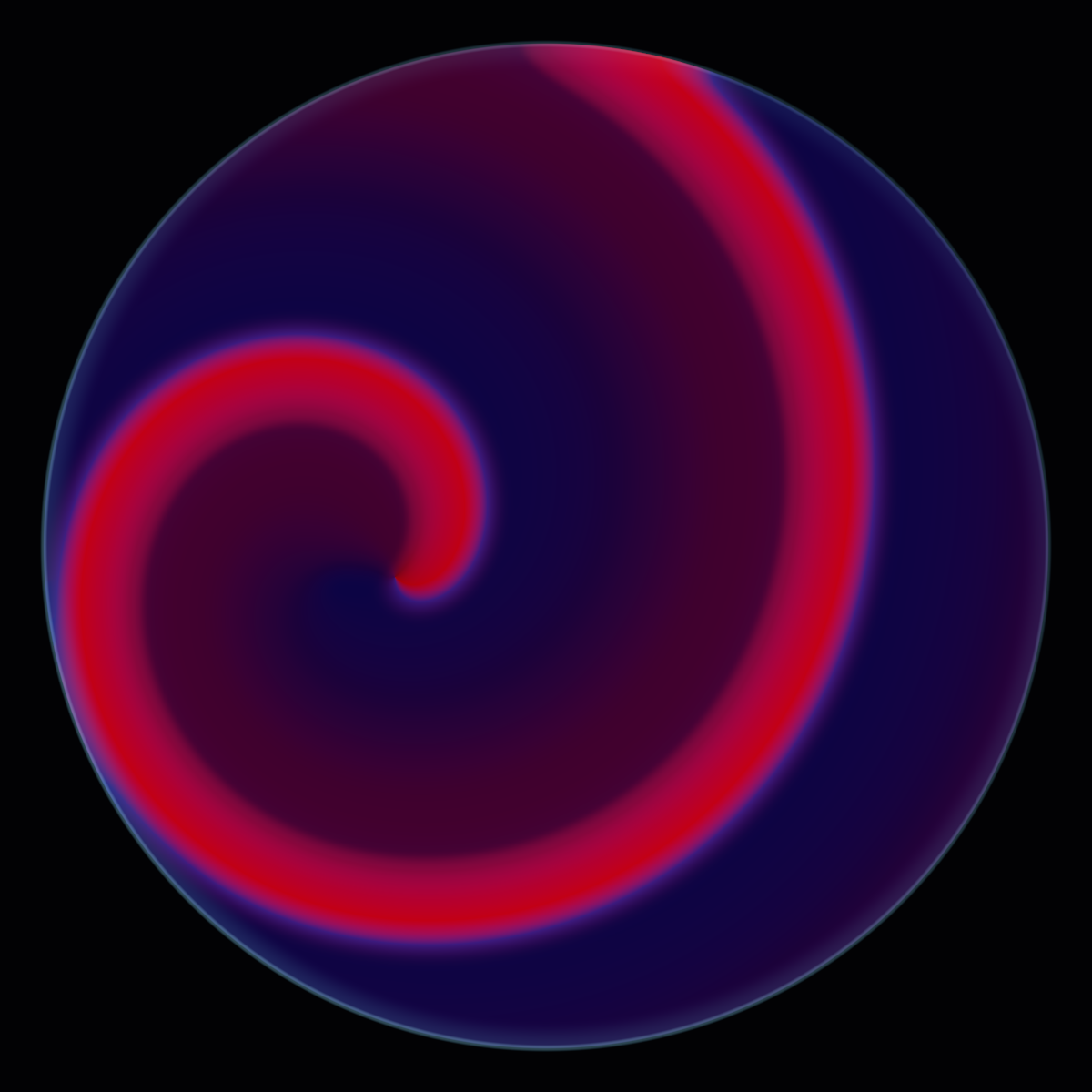
Start here: the Gallery opens on the validated Persistent Single Spiral at its mature checkpoint. In Gentle or Alive motion mode it continues from that exact numerical state; in Still mode it waits, intact, for Play or Step. Switch display styles before opening the Laboratory—the wave should not move merely because its colour mapping changed.
BZ Laboratory V2 · numerical exhibit
Chemical waves, spectacle with receipts
One numerical state can be viewed as a luminous dish, inspected as raw fields, and audited against its calibration record.Gallery · calibrated states only
A dish first. Instruments when you ask.
Mature frames come only from the versioned manifest. Genesis replay remains a separate, explicit action.
Choose a pattern to inspect its manifest status.
- Step
- —
- Model t
- —
- Engine
- asset
Proof · generated evidence
Claims stop where the manifest stops.
This layer reads the same public V2 calibration manifest used by presets, checkpoints and publication records. Empty evidence remains visibly empty.
Persistent Single Spiral
The Gallery stage remains the owner of this run. Proof reads its bounded frame summary; opening this panel neither reconstructs nor resets the field.
No numerical frame has been published by the Gallery stage yet.
Classic Target Rings
Every deterministic Float64 morphology search, convergence, authenticated checkpoint, explicitly scoped implementation-and-display-64 browser parity, display-independence, publication-metadata and exact checkpoint-poster gate passed.
- Observation
- 10.000–14.000
- Grid
- 256²
- Fixed Δt
- 0.0005
- Source
- declared periodic external source
Criteria and measurements
Passed
- finite-state
- three-outward-fronts
Measurements
- grid
- 256
- maximumSignificantPeaks
- 3
- meanWaveSpeed
- 4.86566105769231
- modelTime
- 14
- outwardTrackCount
- 4
- simultaneousThreePeakFraction
- 0.9629629629629629
- wallReflectionTracks
- 0
Persistent Single Spiral
Every deterministic Float64 morphology search, convergence, authenticated checkpoint, explicitly scoped implementation-and-display-64 browser parity, display-independence, publication-metadata and exact checkpoint-poster gate passed.
- Observation
- 2.000–14.000
- Grid
- 256²
- Fixed Δt
- 0.0005
- Source
- finite initial perturbation
Criteria and measurements
Passed
- finite-state
- persistent-rotating-single-core
Measurements
- exactlyOneCoreFraction
- 1
- grid
- 256
- minimumWallDistance
- 8.161370188827547
- modelTime
- 14
- rotationPeriodCv
- 0.004553421293048651
- rotationPeriodMean
- 2.7371865723806916
- rotations
- 4.210468715488337
Spiral Garden
Every deterministic Float64 morphology search, convergence, authenticated checkpoint, explicitly scoped implementation-and-display-64 browser parity, display-independence, publication-metadata and exact checkpoint-poster gate passed.
- Observation
- 2.000–12.000
- Grid
- 256²
- Fixed Δt
- 0.0005
- Source
- finite initial perturbation
Criteria and measurements
Passed
- finite-state
- persistent-three-core-garden
Measurements
- grid
- 256
- minimumCoreCount
- 3
- minimumMeasuredRotations
- 3.620510653105014
- minimumSeparation
- 5.215661511256266
- minimumWallDistance
- 6.93279093641374
- modelTime
- 12
- persistentTrackCount
- 3
Checkpoint fields and measured motion
This panel reads the selected checkpoint directly. It never requests a field snapshot from the live Gallery engine.
Field evidence loads only while Proof is open.
Numerical contract
- Engine
bz-heun-five-point-v2- Display
bz-display-linear-light-v2- Generated by
- scripts/generate-bz-v2-manifest.mjs
- Generated at
- 2026-08-08T12:24:26.141Z
Integrator: Fixed-timestep explicit Heun integration of the declared two-variable Oregonator with fail-fast finite and negativity checks.
Boundary: Five-point Laplacian with explicit circular-domain and active-cell masks; missing neighbours use the declared no-flux rule.
Display contract
Interpolation, palette, exposure, bloom, tone mapping and glass treatment are presentation only. They do not enter the PDE state.
- Oregonator luminous publication profileluminous-composite · fixed rangesLuminous phase and wavefront composite in linear light with fixed ranges; restrained bloom, tone mapping, and glass cues are display only.
- Oregonator scientific publication profilescientific · fixed rangesRaw numerical field on a fixed scientific range; no bloom or chemical-colour claim.
- Schnakenberg scientific publication profilescientific · fixed rangesRaw Schnakenberg u field on a fixed scientific range; the linearly verified diffusion-driven comparator remains distinct from travelling BZ waves.
Convergence and parity
classic-target-rings-validation-v2
Every deterministic Float64 morphology search, convergence, authenticated checkpoint, explicitly scoped implementation-and-display-64 browser parity, display-independence, publication-metadata and exact checkpoint-poster gate passed.
- meanWaveSpeed256² versus 128²: 3.11% / 5.00% tolerance
- meanWaveSpeedΔt 0.0005 versus 0.00025 at 128²: 0.00% / 5.00% tolerance
Browser CPU/GPU fixed-step integration, declared intervention scheduling and display-transform agreement were measured at 64². This is implementation parity only; mature 256² morphology, core rotations and target fronts are established by the authenticated Float64 CPU search, convergence and checkpoint provenance, not by GPU remeasurement.
- base fixed step 64 64² · step 64 max |Δ| 0.000000 · RMS 0.000000
- declared intervention schedule 64 64² · step 3,002 max |Δ| 0.000005 · RMS 0.000000
persistent-single-spiral-validation-v2
Every deterministic Float64 morphology search, convergence, authenticated checkpoint, explicitly scoped implementation-and-display-64 browser parity, display-independence, publication-metadata and exact checkpoint-poster gate passed.
- rotationPeriodMean256² versus 128²: 0.03% / 2.00% tolerance
- rotationPeriodMean256² Δt 0.0005 versus 96² Δt 0.00025 refinement: 0.42% / 5.00% tolerance
Browser CPU/GPU fixed-step integration, declared intervention scheduling and display-transform agreement were measured at 64². This is implementation parity only; mature 256² morphology, core rotations and target fronts are established by the authenticated Float64 CPU search, convergence and checkpoint provenance, not by GPU remeasurement.
- base fixed step 64 64² · step 64 max |Δ| 0.000000 · RMS 0.000000
- declared intervention schedule 64 64² · step 902 max |Δ| 0.000001 · RMS 0.000000
spiral-garden-validation-v2
Every deterministic Float64 morphology search, convergence, authenticated checkpoint, explicitly scoped implementation-and-display-64 browser parity, display-independence, publication-metadata and exact checkpoint-poster gate passed.
- minimumMeasuredRotations256² versus 96²: 0.78% / 5.00% tolerance
- minimumMeasuredRotations256² Δt 0.0005 versus 64² Δt 0.00025 refinement: 0.89% / 5.00% tolerance
Browser CPU/GPU fixed-step integration, declared intervention scheduling and display-transform agreement were measured at 64². This is implementation parity only; mature 256² morphology, core rotations and target fronts are established by the authenticated Float64 CPU search, convergence and checkpoint provenance, not by GPU remeasurement.
- base fixed step 64 64² · step 64 max |Δ| 0.000000 · RMS 0.000000
Browser performance evidence
No measured browser performance report is published yet.
One field, two views
Scientific view shows the dimensionless model fields on fixed ranges. Ferroin-inspired view is a representative colour mapping, not a measurement of ferroin or ferriin concentration. Luminous view combines a fixed phase coordinate with measured front information so that narrow waves remain legible. Interpolation, exposure, bloom, tone mapping and the glass rim affect presentation only. No ring, core or spiral is generated by the renderer.
What is physics, and what is presentation?
| Numerical model | Display only |
|---|---|
| Oregonator or Schnakenberg reaction terms | Mask-aware visual interpolation |
| Diffusion coefficients and five-point Laplacian | Palette and representative colour |
| Fixed timestep and Heun integration | Exposure and saturation |
| No-flux or periodic boundary | Front-linked bloom |
| Initial numerical state | ACES tone mapping and sRGB transfer |
| Declared pacemaker schedule | Glass rim and meniscus cue |
| Domain and obstacle masks | Labels and explanatory overlays |
Changing the right-hand column cannot reset or alter the left-hand state. The Proof layer exposes the validation record, checkpoint provenance, convergence comparisons and finite-time claim boundaries behind each Gallery badge.
Uses the speech voice supplied by your browser or device.
1. A quiet dish that starts drawing
The first useful distinction is between a colour changing everywhere together and a coloured state moving through space. A well-mixed oscillating reaction can do the former. A shallow unstirred layer can do the latter because one patch may be excited while its neighbour is recovering. The visible line is an excitation front, not paint being transported as a rigid ring.
Three observations keep the opening honest. The front takes time to cross the dish. Two fronts usually annihilate when they collide. After a front passes, the same place cannot immediately support another. Those are clues to an excitable or oscillatory medium with a refractory history. They are not, by themselves, the classical test for a Turing instability.
2. The chemical clock
In a well-mixed vessel, every small region is continually brought into contact with the rest. Spatial gradients are suppressed, so a useful first approximation has only time-dependent state variables. Feedback can carry that state around a closed orbit in phase space: one process rises, activates or depletes another, an inhibitory process catches up, and recovery prepares the system for another excursion.
This repeating orbit is a limit cycle, not equilibrium. At equilibrium the macroscopic state is constant. On a limit cycle the state keeps changing, even though it eventually revisits the same sequence. A clock hand returning to twelve has not stopped; nor has chemistry returning near an earlier pair of concentrations reached equilibrium.
The well-mixed control keeps every active cell identical, so its spatial variance remains at round-off scale while the local state changes. It is a control for distinguishing a temporal clock from a travelling wave; the three validated Gallery claims belong to separate spatial presets and their declared finite observation windows.
The well-mixed control makes the distinction visible. Every numerical cell begins identically, so diffusion has nothing to transport. The dish changes as one, while the local and traces loop around the phase portrait. Pause on two moments with similar colour and inspect both fields: a display colour can conceal that the full chemical state differs. That is why one coloured channel is a poor substitute for phase space.
3. Boris Belousov and the unwelcome oscillation
Boris Belousov found an oscillating chemical reaction in the early 1950s. The result arrived in a scientific climate where repeated change in a closed, homogeneous reaction was easy to mistake for faulty observation or inadequate mixing. His attempts to publish a full account met rejection. A short Russian report, Periodicheski deistvuyushchaya reaktsiya i ee mekhanizm—“Periodically acting reaction and its mechanism”—appeared in a collection dated for 1958 and published by Medgiz in 1959, on pages 145–147.
Alexander Pechenkin reconstructs the publication history from archival material in “B. P. Belousov and His Reaction”. It needs no invented dialogue: an observation can be correct before its mechanism is persuasive.
Belousov discovered the oscillation. He did not write the Oregonator or the two partial differential equations running below. Those came through several later acts of modelling, each of which retained some chemical logic and discarded some detail.
4. Anatol Zhabotinsky gives the clock a geography
During the 1960s Anatol Zhabotinsky investigated and developed the reaction systematically, including its spatial behaviour. In a shallow unstirred layer, local regions could occupy different chemical states. Excitation bands travelled; concentric waves and spirals made temporal organisation visible as a moving map. Zaikin and Zhabotinsky’s 1970 Nature paper on concentration-wave propagation and Field and Noyes’s 1972 explanation of spatial band propagation belong to the experimental and theoretical route by which these observations became internationally legible.
The important word is unstirred. Mixing forces locations towards a common state. Without that enforced agreement, local kinetics can get out of phase and diffusion can couple nearby patches. One place excites its neighbour, which excites the next: a field of clocks whose disagreements propagate.
Arthur Winfree’s “Spiral Waves of Chemical Activity” showed how seriously the geometry itself deserved to be taken. A broken wave could form a persistent spiral rather than merely a damaged circle. The pattern was not an ornamental afterthought to the chemistry; it was an organised dynamical object.
5. Why the second law has not left the building
Oscillating colour can suggest a reaction running forwards and backwards for free. It is doing no such thing. The BZ reaction is a dissipative, far-from-equilibrium process. Chemical free energy is consumed while intermediate states rise and fall; entropy production has not been suspended for aesthetic reasons.
A closed batch ages. Its usable reactants are depleted, products accumulate, and oscillations eventually cease or change character. The reduced equations here hold their dimensionless parameters approximately fixed over a chosen observation interval. They can therefore sustain behaviour longer than a particular batch would. That is a modelling decision, not perpetual motion, and it is one reason the export calls itself a model experiment rather than a laboratory forecast.
6. From ODE to PDE
Begin with one well-mixed local clock:
In plain language: and say how reaction changes the two state variables at one location. There is no left, right or neighbouring pixel. In the laboratory, the well-mixed preset isolates this part. What it omits is transport, vessel geometry and every chemical species not represented by and .
Now allow each location to have its own state and let nearby locations exchange material:
In plain language: reaction changes a location according to its own state; diffusion changes it according to spatial curvature relative to its neighbours. A peak tends to lose material and a hollow tends to gain it. Use Reaction only and Diffusion only to separate the contributions. These equations still omit fluid flow: diffusion is molecular transport down gradients, not a miniature stirring animation.
Calling diffusion “blur” misses its accounting. A blur is a picture operation. A Laplacian plus a boundary condition is a transport law. In a no-flux dish it redistributes a field without allowing it to cross the wall, apart from numerical error.
7. The Oregonator came later
The historical and modelling hierarchy is:
real BZ chemistry
↓
Field–Körös–Noyes mechanism
↓
Oregonator reduction
↓
Tyson–Fife two-variable spatial model
↓
this browser discretisation
Field, Körös and Noyes gave a detailed mechanistic account of temporal oscillation in 1972. Field and Noyes then compressed essential feedback into the Oregonator and analysed its limit cycle in 1974. Their accompanying work connected the model to migrating bands quantitatively. John Tyson and Paul Fife’s 1980 target-pattern paper supplied the later two-variable spatial reduction used as the principal ancestor here.
A reduction is useful because two fields can be plotted, probed and understood in phase space. It is limited for the same reason. The fields are dimensionless proxies, not an inventory of molecules, and do not reproduce every FKN pathway.
One declaration matters to specialists. A common Tyson–Fife spatial form treats the slow field as non-diffusing. This exhibit writes an explicit term and permits or a tested non-zero value. That is a transparent generalisation for controlled model experiments, not a claim that every preset or diffusion coefficient was reported in the 1980 paper. Presets are labelled as finite-time validated or as candidates according to their recorded browser calibration; neither label turns them into literature values.
8. The two equations, term by term
The principal model is the dimensionless two-variable Oregonator in the form
In plain language: is the fast, activator-like field and is the slower recovery or catalyst-like field. Diffusion moves each field between neighbours. The bracket can make rise sharply or be suppressed by . The term makes follow excitation and then relax. Paint Excite to cross a local threshold; use Recover to move a patch towards the slower state; switch the ledger between reaction, diffusion and net change. The equations omit the complete reaction network, laboratory units, batch depletion and fluid motion.
Every symbol earns its place:
- redistributes the fast field. At a local peak it is usually negative; in a surrounding hollow it is positive.
- does the same for the recovery field when . Setting makes recovery local rather than spatially transported.
- supplies nonlinear self-activation at moderate and restrains it as approaches the selected scale near one.
- is the recovery-dependent inhibitory contribution. For it pulls the fast field down more strongly as or rises.
- makes the kinetics fast when is small. It also makes careless timesteps especially expensive.
- is a small kinetic threshold parameter in the reduction. It regularises the denominator and changes the low- geometry; it is not a quality setting.
- drives upward when excitation exceeds recovery and downward when recovery has caught up.
The equation ledger below evaluates these contributions at the probe. It is not a symbolic decoration: reaction plus diffusion equals the reported instantaneous net change, subject to floating-point precision.
Interactive equation ledger
Separate reaction from transport
- Reaction
- +2.58435
- Diffusion
- -0.08000
- Net change
- +2.50435
- Reaction
- +0.20000
- Diffusion
- 0.00000
- Net change
- +0.20000
9. Excitability, threshold and refractory time
Imagine a row of doorbells in a street, each wired to its neighbours and each requiring time to reset. A weak tap may do nothing. A sufficient press rings one bell, its coupling triggers the next, and a signal travels. The bell just rung cannot ring again immediately. The analogy is useful only up to this point: the medium is not a street, and a dimensionless chemical field is not a neuron in a novelty hat.
With diffusion turned off, the local motion can be read from nullclines, where one time derivative vanishes. Ignoring spatial terms, they include
In plain language: on the first curve, is momentarily neither rising nor falling; on the second, is momentarily balanced. Between the curves, the signs of and point the state around phase space. Use a probe and a sub-threshold pulse, then a stronger pulse. The first returns near the resting branch; the second makes a large excursion before recovery. The curves describe this reduced local system only—they are not direct concentration measurements.
In space, a recovered patch ahead of a front can be pushed across threshold by diffusive input from an excited neighbour. Behind the front, elevated recovery suppresses immediate re-excitation. That refractory wake gives the wave direction and supplies the spiral with memory. Phase matters: two pixels of similar displayed colour may respond differently because their hidden values differ.
10. Target waves
A target pattern needs a source that fires repeatedly. In this model the validated source is a declared local state-reset intervention with period 1.5 model-time units, active from through . Each event can launch a radial front into recovered territory. Because the circumference grows as the front expands, a ring becomes geometrically larger without material being carried outward as a hoop.
If the front speed is and the source period is , the distance between successive rings is approximately
In plain language: a faster front or a slower clock puts rings farther apart. The relation is an operational wave estimate, not a promise that curvature, refractory variation and finite boundaries leave perfectly constant.
For the promoted 256² target run, the declared to window contained three significant radial peaks in 96.3% of samples. The minimum measured spacing was 12.506 dimensionless length units, four tracks moved outward with mean speed 4.866, peak order was preserved, and no reflected wall track was counted as a new wave. The 128² refinement and timestep-halved controls preserved the repeated outward-front result.

The ring moves. Test that sentence by pausing twice at equal model-time intervals and recording the radius of one identified crest. A merely flashing set of static annuli would fail the experiment. Then install the logged pacemaker and ask separately whether later crests repeat.
11. How a broken wave becomes a spiral
A complete closed front has no free endpoint. Cut a finite gap and two ends appear. Near either end, one side faces recovered, excitable medium while the other borders its own refractory wake. Propagation is therefore asymmetric. Curvature slows and turns the free edge; recovery continues behind it; the tip curls around a small core. If the parameter regime supports it, rotation persists and emits a spiral wave.
The diagram separates the excited front, refractory wake, free end and curling sequence. The live Cut front tool changes the model fields over a finite stroke. It does not rotate a texture, impose an angular colour map or paste in a spiral. A genuine test is local: follow the tip, watch the phase portrait cycle around it, and verify that newly excited material continually replaces the old front.
The promoted single-spiral preparation starts with a plane wave and performs one declared half-plane reset at , leaving a free end rather than painting a curved arm. From to , one same-charge phase-winding core was tracked at every sample. The annular front orientation accumulated 4.210 rotations, its mean measured period was 2.7372 with coefficient of variation 0.00455, and the core retained at least 8.161 dimensionless units of wall clearance. The 128² and 96² refinements and the timestep-halved run preserved the core and approximate period.

The core is not a physical peg. It is the small region around which the wave tip rotates, determined by front curvature, kinetics and recovery. Add an impermeable obstacle and the wave may pin to that geometry; remove or move the obstacle and you have changed the experiment, not discovered a more photogenic phase.
The third Gallery regime begins from three declared phase singularities. Across to , three continuously associated cores persisted for the full ten-unit window; the least-rotating track completed 3.621 rotations, minimum pairwise separation was 5.216, and minimum wall clearance was 6.933. A 96² refinement and a timestep-halved control preserved the three-core result.

12. Chemical waves are not water waves
Two small-amplitude water waves can pass through one another because their displacements approximately superpose. Two excitation fronts in this medium ordinarily cannot. Each consumes the immediate ability of the medium to fire and leaves a refractory wake. When fronts meet, there is no recovered territory on the far side of either front. Both terminate.
The collision control launches opposing fronts and records active length before and after contact. If they pass through and continue unchanged, the explanation has failed—or the model is in a different regime. Annihilation is not a display fade; it is a consequence of local state.
13. What stirring removes
Physical stirring couples chemistry to advection and complicated fluid motion. The browser does not pretend to solve that problem. Its Stir action performs a declared homogenisation: it computes the active-area mean of and of , replaces every accessible dish cell with those means, and leaves the circular wall and obstacle mask intact. Apart from round-off, the two active-area means are preserved while spatial variance collapses.
This erases concentration gradients, phase differences, fronts and spiral tips. It need not stop temporal oscillation. If the resulting mean state lies in an oscillatory regime, the dish may continue changing globally, as one clock again. Measure variance before and after, then watch the active-area mean. The honest question is not “Did stirring kill the reaction?” but “Did it erase the geography while leaving the clock?”
14. Turing’s 1952 question
Alan Turing asked how an initially homogeneous biological system might develop spatial differences through ordinary physical laws. In “The Chemical Basis of Morphogenesis”, published in 1952, he proposed reacting and diffusing morphogens as one possible mathematical mechanism. A homogeneous state could be stable when every location changed together yet unstable to selected spatial disturbances once diffusion joined the kinetics.
Turing did not discover zebra stripes in a bottle, and the BZ experiment was not a direct response to his paper. The chemical-oscillation and morphogenesis histories developed largely independently before being joined within the wider study of nonlinear reaction–diffusion systems. His original analysis also covered more dynamical possibilities than the later shorthand “stationary spots and stripes” suggests.
Turing died in 1954; the coroner’s verdict was suicide, although the full circumstances have remained a subject of later discussion. That fact belongs to an accurate biography, but it supplies neither the mechanism nor a promotional hook.
15. The classical Turing test
Write a general two-field system as
In plain language: and are local reactions; the Laplacians couple locations. The classical stationary Turing question is not whether a finished field has spots. It is whether diffusion makes a spatial mode grow around a reaction-stable homogeneous equilibrium. This linear test describes the onset near that equilibrium; it does not predict every nonlinear detail of the mature pattern.
The comparator uses the Schnakenberg model exactly as
with homogeneous equilibrium
In plain language: the term transfers local influence between the fields with opposite signs, and supply the selected kinetics, and sets their overall timescale. At both reaction terms vanish. Start Stable uniform to test whether numerical noise remains quiet; then choose the finite-mode Turing comparator and inspect its dispersion status before calling the mature field a spot, stripe or labyrinth. These are dimensionless comparator fields, not named morphogens.
Linearise the reactions at the equilibrium. Their Jacobian is
For a spatial Fourier mode of wave number , diffusion changes it to
In plain language: first inspect the eigenvalues at . Their real parts must be negative, so a spatially uniform disturbance decays. Then scan . A classical diffusion-driven preset must have a finite non-zero band where the largest real part becomes positive. The fastest-growing predicts . The later field spectrum should show a compatible peak; if it does not, the panel says no trustworthy measured wavelength rather than recruiting a convenient bump.
Live Schnakenberg stability inspector
Does diffusion create a growing spatial mode?
Largest real eigenvalue: -0.10000
Maximum sampled growth: 0.05719
Both necessary linear tests pass.
Eigenvalues are evaluated analytically for each sampled k; band endpoints are linearly interpolated between neighbouring samples. This is a linear onset test, not a measurement of the mature field.
| Quantity | Result | Why it matters |
|---|---|---|
| Homogeneous equilibrium | u* = 1.000, v* = 0.900 | Both local reaction terms vanish here. |
| Reaction Jacobian | [0.800, 1.000, -1.800, -1.000] | Trace -0.200; determinant 1.000. |
| Reaction eigenvalues | -0.1000 + 0.9950i; -0.1000 − 0.9950i | Both real parts must be negative at k = 0. |
| Positive-growth band | 4.47 < k < 7.07 | A classical diffusion-driven onset needs growth at non-zero k. |
| Fastest mode | k = 5.646 | Predicted λ = 1.113. |
| Grid resolution | Fastest mode is resolved | Grid Nyquist limit: 20.11. |
In plain language. First ask whether a well-mixed nudge dies. Then ask whether diffusion makes some finite spatial wavelength grow. Only the combination—stable at k = 0, unstable for a band with k > 0—earns the classical diffusion-driven label used here.
16. BZ waves are related to Turing patterns—but not identical
Both systems combine local nonlinear change with spatial diffusion. That shared grammar explains the family resemblance. It does not make their sentences interchangeable.
| Question | BZ / two-variable Oregonator here | Classical Turing / Schnakenberg here |
|---|---|---|
| Base state | Oscillatory local state or excitable rest state | Homogeneous reaction equilibrium |
| Instability or trigger | Local oscillation, finite excitation or wave source | Diffusion destabilises an otherwise reaction-stable equilibrium |
| Temporal signature | Periodic excitation and recovery remain conspicuous | Growth may settle towards a relatively stationary morphology |
| Spatial motion | Fronts travel; target rings expand; spirals rotate | Selected modes amplify broadly rather than sweep as one refractory front |
| Refractory state | Central to direction, collision and spiral recovery | Not the defining ingredient of the classical test |
| Collision | Excitation fronts usually annihilate | Domains compete and coarsen; there is no universal front-annihilation rule |
| Wavelength | Often set by wave speed × firing period, with curvature corrections | Selected by a finite band in the dispersion relation |
| Common mature view | Moving targets, spirals and broken waves | Spots, stripes or labyrinths that become comparatively stationary |
| Biological analogy | Cardiac, calcium or cyclic-AMP excitation waves | Morphogen-driven pigmentation or tissue-spacing hypotheses |
| Diagnostic | Follow fronts, phase and refractory recovery through time | Verify stability and positive growth at some |

The nuance matters in both directions. Reaction–diffusion theory contains stationary, oscillatory and mixed instabilities; Turing’s paper was broader than its modern postcard. Extended BZ systems can enter Turing-like or mixed regimes. But a familiar rotating spiral should not be renamed without analysing its base state and growing modes. Celebrity is not a stability criterion.
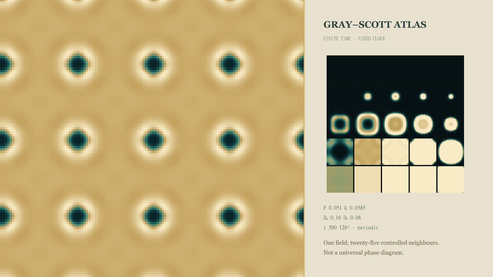
The Reaction–Diffusion Atlas investigates the different Gray–Scott model and goes deeper into finite-amplitude patterning, linear stability and numerical convergence. This laboratory is its companion, not its replacement.
17. Where biology rhymes with the dish
There are at least two different biological rhymes, and combining them produces a very confident muddle.
First are excitable waves. Cardiac excitation, intracellular or intercellular calcium waves, and cyclic-AMP signalling in aggregating Dictyostelium can propagate through media with threshold and recovery. Experiments have directly visualised concentric and spiral cyclic-AMP waves organising Dictyostelium mounds. The useful claim is shared mathematical structure: local activation, coupling and refractoriness. The cells, channels and regulatory networks are not the BZ chemistry in disguise.
Second are morphogenic reaction–diffusion mechanisms. Work on fish pigmentation, hair-follicle spacing and other developing tissues has tested activator–inhibitor or related models against perturbation and molecular evidence. Kondo and Miura’s 2010 review explains why dynamic pattern repair and wavelength behaviour can be more informative than resemblance. The WNT–DKK study of hair-follicle spacing, for example, joined a reaction–diffusion model to molecular intervention rather than announcing victory because a simulation had dots.
Biological plausibility therefore climbs an evidence ladder: a visual match; a dynamical prediction; measured components and interactions; perturbations that move the pattern as predicted; and alternatives that fare worse. The Brownian Motion Laboratory provides a useful contrast: random molecular-scale transport can underlie diffusion, but an organised excitation wave is a collective field phenomenon, not a crowd of coloured particles marching in formation.
18. A later chemical bridge
In 2014 Nathan Tompkins, Ning Li, Camille Girabawe, Michael Heymann, G. Bard Ermentrout, Irving R. Epstein and Seth Fraden reported “Testing Turing’s Theory of Morphogenesis in Chemical Cells”. Their system was an oil emulsion of coupled aqueous droplets containing BZ reactants: synthetic chemical cells, not living cells. Diffusive coupling allowed the investigators to compare a controlled cellular chemical experiment with structures from Turing’s analysis.
They observed five of the six structures discussed in the relevant prediction and found an additional mixed spatial–temporal structure in two-dimensional hexagonal arrays, which required extending the treatment to heterogeneity. The experiment is a genuine bridge because it tests compartmentalised reaction–diffusion with known chemistry and coupling. It does not prove that every embryo uses the same mechanism, nor does it retroactively convert every ordinary BZ spiral dish into a stationary Turing pattern.
19. How the browser calculates the dish
The simulation replaces a continuous sheet with a finite square grid clipped by a circular active mask. At an interior cell the five-point Laplacian is
In plain language: compare one cell with its four axial neighbours. At the circular wall or an obstacle, a missing neighbour contributes the centre value, enforcing the discrete no-flux rule used here. Nothing communicates with hidden pixels outside the dish. The approximation omits diagonal coupling at this order and becomes a better account of the declared continuum problem only under resolution checks.
Time advances by fixed-step Heun integration. If contains both fields and contains reaction plus diffusion,
In plain language: make one Euler prediction, evaluate the slope again there, then correct using the average slope. Speed changes how many fixed steps are attempted per wall-clock second; it never secretly enlarges . The normal solver does not clip an unstable state back into a pretty range.
Raw WebGL2 fragment shaders carry out those passes over floating-point textures. One texture holds the current state, a predictor pass writes another, a correction pass writes the next, and the references swap. A separate display shader maps and to colour. The graphics processor is therefore evaluating a numerical stencil at every active cell, not merely tinting an animation. The CPU reference engine uses the same equations for calibration and small-grid comparisons.
The Living Pigment Studio uses related shader craft for expressive painting. Here the numerical state, display palette and intervention log are more sternly separated: changing the palette must leave the field checksum alone.
20. How arithmetic can counterfeit chemistry
A plausible spiral can be numerically false. A timestep too large for the fast kinetics or diffusion scale may amplify error. A coarse grid may pin a front or erase its core. A square wraparound seam can masquerade as communication across a circular vessel. Hidden clipping can keep a failing field bounded. Comparing a coarse run at time 40 with a fine run at time 60 rewards whichever transient happens to look more convincing.
GPU precision adds another layer. Floating-point texture formats and shader arithmetic need not reproduce Float64 CPU arithmetic bit for bit. Agreement is therefore measured by declared errors and field summaries at equal model time, with tolerances tied to the precision tier. Sensitive nonlinear trajectories may diverge eventually even when short-time convergence is sound.
The checks below keep the comparisons controlled:
- timestep against at equal model time;
- coarse against fine grid at the same physical domain and time;
- CPU against GPU from identical initial arrays over a short interval;
- a deliberately unsafe timestep isolated from the production state and stopped on non-finite or declared raw-limit failure.
Controlled numerical audit
Can arithmetic counterfeit the chemistry?
Timestep versus half timestep
not runCompare Δt with Δt/2 at exactly the same model time.
Coarse versus fine grid
not runCompare 32² and 64² grids over one declared domain and time.
Unsafe timestep isolation
not runConstruct a step above the explicit five-point diffusion bound and require rejection.
The checks run in isolated Float64 CPU fields and never touch the live dish.
Accessible results table
| Check | State | Result | Interpretation |
|---|---|---|---|
| Timestep versus half timestep | idle | not run | Compare Δt with Δt/2 at exactly the same model time. |
| Coarse versus fine grid | idle | not run | Compare 32² and 64² grids over one declared domain and time. |
| Unsafe timestep isolation | idle | not run | Construct a step above the explicit five-point diffusion bound and require rejection. |
Convergence does not mean every pixel becomes identical across resolutions. It means a defensible error measure, wave speed, period, spectral peak or other observable approaches agreement as the discretisation is refined. The nearby Double-Pendulum Atlas offers the complementary warning: in nonlinear dynamics, deterministic equations and reproducible initial conditions do not guarantee indefinitely coincident trajectories.
21. Experiments to try
Start the well-mixed clock. Set a uniform oscillatory preset and keep every cell identical. Support: the spatial variance stays near zero while and trace a bounded cycle. Contradiction: coherent fronts appear without any spatial difference or intervention.
Inspect the pacemaker. Select Classic Target Rings and record successive crossings at one radius. Support: each crest reaches the probe later than the previous radial location and the measured spacing is compatible with speed × period. Contradiction: rings flash everywhere at once.
Cut a front. Let a travelling front establish a refractory wake, then make one finite cut. Support: a free tip curls and continually advances into recovered medium. Contradiction: a spiral graphic rotates while the phase and recovery fields remain fixed.
Add an obstacle. Put an impermeable disk ahead of a front. Support: no flux crosses the mask; the front bends around it or pins under a suitable setup. Contradiction: the hidden obstacle interior transmits excitation to the far side.
Collide two waves. Launch opposing fronts as an exploratory Laboratory run. Support: both disappear at contact because the encounter leaves no recovered continuation. Contradiction: the fronts pass through with unchanged identity as linear ripples would. This is not one of the three promoted Gallery claims unless its own recorded criteria are later added to the manifest.
Stir and then watch. Record active-area means and variances, then press Stir once. Support: means are preserved within tolerance, variances collapse, and a global oscillation may continue. Contradiction: the action injects a new mean state or claims to solve fluid vortices.
Compare with the Turing model. Run live BZ and the analytically classified Schnakenberg comparator side by side. Support: the BZ front travels while the comparator selects a finite wavelength and its inspector shows stable with growth at . Contradiction: classification rests only on whether both pictures contain spots.
Halve the timestep. Replay from the same seed and intervention log to the same model time. Support: probe periods, wave position and summary errors move towards agreement. Contradiction: a production preset survives only because clipping conceals a timestep failure.
22. What this model does not simulate
The browser does not contain the complete Field–Körös–Noyes reaction network, every chemical species, quantitative laboratory concentrations, calibrated spectroscopy or every branch of catalyst chemistry. Its and are dimensionless model fields. A pixel is not one molecule, however earnestly it glows.
It also omits fluid advection, convection, meniscus-driven flow, bubbles or gas evolution, heat transport, evaporation, three-dimensional depth, exact batch depletion and vessel contamination. Stir is mean-preserving homogenisation, not computational fluid dynamics. Obstacles are impermeable masks, not pieces of laboratory material with surface chemistry.
The biological comparator omits gene regulation, cell mechanics, tissue growth and anatomical geometry. It is not a universal theory of animal markings. The Schnakenberg model demonstrates a mathematically classifiable diffusion-driven mechanism; it does not identify a morphogen pair in a particular organism. These omissions are not small print beneath an otherwise quantitative chemical claim. They define what the exhibit is.
23. Safety
This is a numerical exhibit, not a home experiment. Real Belousov–Zhabotinsky demonstrations can involve strong acid, oxidising chemistry, catalysts and other hazardous reagents. No quantities, concentrations or mixing instructions are provided here. A physical demonstration belongs in a properly equipped, supervised laboratory under an approved procedure; a browser’s Reset button is not transferable to a laboratory bench.
24. References
Primary papers are linked by DOI; the historical bibliography is given explicitly because the 1959 collection and its date are easily garbled.
- B. P. Belousov, “Periodicheski deistvuyushchaya reaktsiya i ee mekhanizm” [“Periodically acting reaction and its mechanism”], Sbornik referatov po radiatsionnoi meditsine, 1958 (Moscow: Medgiz, published 1959), pp. 145–147. An English translation, titled “A Periodic Reaction and Its Mechanism”, appears in R. J. Field and M. Burger (eds.), Oscillations and Traveling Waves in Chemical Systems (Wiley, 1985), pp. 605–613.
- A. Pechenkin, “B. P. Belousov and His Reaction”, Journal of Biosciences 34 (2009), 365–371. Historical study using archival evidence.
- A. M. Zhabotinsky, “A History of Chemical Oscillations and Waves”, Chaos 1 (1991), 379–386.
- A. N. Zaikin and A. M. Zhabotinsky, “Concentration Wave Propagation in Two-Dimensional Liquid-Phase Self-Oscillating System”, Nature 225 (1970), 535–537.
- R. J. Field, E. Körös and R. M. Noyes, “Oscillations in Chemical Systems. II. Thorough Analysis of Temporal Oscillation in the Bromate–Cerium–Malonic Acid System”, Journal of the American Chemical Society 94 (1972), 8649–8664.
- R. J. Field and R. M. Noyes, “Explanation of Spatial Band Propagation in the Belousov Reaction”, Nature 237 (1972), 390–392.
- R. J. Field and R. M. Noyes, “Oscillations in Chemical Systems. IV. Limit Cycle Behavior in a Model of a Real Chemical Reaction”, Journal of Chemical Physics 60 (1974), 1877–1884.
- R. J. Field and R. M. Noyes, “Oscillations in Chemical Systems. V. Quantitative Explanation of Band Migration in the Belousov–Zhabotinskii Reaction”, Journal of the American Chemical Society 96 (1974), 2001–2006.
- A. T. Winfree, “Spiral Waves of Chemical Activity”, Science 175 (1972), 634–636.
- J. J. Tyson and P. C. Fife, “Target Patterns in a Realistic Model of the Belousov–Zhabotinskii Reaction”, Journal of Chemical Physics 73 (1980), 2224–2237.
- A. M. Turing, “The Chemical Basis of Morphogenesis”, Philosophical Transactions of the Royal Society B 237 (1952), 37–72.
- S. Sick, S. Reinker, J. Timmer and T. Schlake, “WNT and DKK Determine Hair Follicle Spacing Through a Reaction-Diffusion Mechanism”, Science 314 (2006), 1447–1450.
- S. Kondo and T. Miura, “Reaction–Diffusion Model as a Framework for Understanding Biological Pattern Formation”, Science 329 (2010), 1616–1620.
- N. Tompkins, N. Li, C. Girabawe, M. Heymann, G. B. Ermentrout, I. R. Epstein and S. Fraden, “Testing Turing’s Theory of Morphogenesis in Chemical Cells”, Proceedings of the National Academy of Sciences 111 (2014), 4397–4402.
25. FAQ
The twelve questions immediately following this article give the short version without quietly changing the model: what oscillates, why rings travel, how spirals begin, what stirring removes, what Turing proposed, and why this page supplies no chemical recipe. Their answers are generated from the same publication metadata as the page’s FAQ structured data, so the visible and machine-readable claims cannot wander apart.
Finish with one concrete observation. In the Gallery, pause Persistent Single Spiral and switch between raw , phase, ferroin-inspired and luminous views. The front must remain at the same numerical position. Then replay genesis: a plane wave and one declared cut must produce the evolving free tip without any renderer inventing curved geometry. The Proof layer records the finite window in which that core persisted and the surrounding front completed 4.210 measured rotations.
Quick reference and FAQ
A chemical clock can oscillate everywhere at once. Let neighbouring places differ, add diffusion, and the same local timing can travel as rings and spirals. This laboratory separates those moving BZ waves from classical Turing patterns, then exposes the equations and numerical tests behind both.
Key Terms
- Belousov–Zhabotinsky reaction
- Chemical oscillator
- Oregonator
- Tyson–Fife model
- Excitable medium
- Target wave
- Spiral wave
- Refractory state
- Reaction–diffusion equation
- Schnakenberg model
- Turing instability
- Dispersion relation
- No-flux boundary
- Heun method
- Numerical convergence
Frequently asked questions
What is the Belousov–Zhabotinsky reaction?
It is a family of far-from-equilibrium oscillating chemical reactions. Feedback among reaction pathways can make measurable chemical states change repeatedly while the batch consumes free energy. In a shallow unstirred medium, local reaction and diffusion can also support travelling target and spiral waves.
Why does its colour oscillate?
The visible indicator responds to a chemical state, often an oxidation state, whose abundance changes as coupled feedback processes alternately accelerate and inhibit one another. The colour cycle records those changing states; it does not mean the overall reaction reverses or revisits equilibrium.
Why do rings form in an unstirred dish?
A repeatedly excited pacemaker can launch a front into recovered neighbouring medium. Diffusion couples nearby locations, so the excitation moves outwards; repeating the event produces successive circular fronts. The rings travel through the dish rather than appearing simultaneously in place.
How does a spiral begin?
A travelling front must acquire a free end, for example when part of it is cut or blocked. Recovered medium lies ahead while refractory medium lies behind. That asymmetric neighbourhood makes the free end curl, and continued excitation and recovery can sustain a rotating spiral tip.
Why do colliding waves disappear?
Each excitation front leaves a refractory wake that cannot immediately support another front. When two fronts meet, each encounters the other’s recently excited material, so neither can continue through. Their annihilation distinguishes these waves from ordinary linear water waves.
What does stirring do?
Stirring removes spatial concentration and phase differences, so fronts and spirals disappear. A well-mixed oscillatory system may still change globally afterwards. The browser’s Stir action is an explicit homogenisation of the two fields, not a simulation of fluid flow.
Is a BZ spiral a Turing pattern?
Usually not in the classical stationary sense. Familiar BZ spirals are rotating waves in oscillatory or excitable media. A classical Turing pattern requires a homogeneous reaction equilibrium stable at zero wave number but destabilised by diffusion over a non-zero band. Both belong to reaction–diffusion theory, but their diagnostics differ.
What is the Oregonator?
The Oregonator is a compact mathematical reduction derived from the Field–Körös–Noyes account of BZ chemistry. It preserves selected feedback needed for oscillation and excitability while omitting many species and elementary reactions. This exhibit uses a later two-variable spatial reduction associated with Tyson and Fife.
Did Belousov write these equations?
No. Boris Belousov discovered the oscillating reaction in the early 1950s and published a short account in 1959. The Field–Körös–Noyes mechanism, Oregonator, and Tyson–Fife two-variable spatial model were developed later by other researchers.
What did Turing propose?
In 1952 Alan Turing proposed a mathematical mechanism by which reacting and diffusing morphogens could amplify spatial differences in an initially homogeneous system. The classical stationary case has a reaction-stable equilibrium that diffusion destabilises at selected non-zero wavelengths, though his original analysis considered a broader set of behaviours.
Is this a quantitative chemical simulation?
No. It is a dimensionless reduced-model laboratory for mechanisms, numerical experiments, and comparisons. Its u and v fields are not calibrated measurements of named molecules, and its presets are browser-calibrated model regimes rather than recipes or quantitative reconstructions of a particular batch.
Is the real reaction safe to reproduce at home?
No. Real BZ demonstrations can involve strong acid, oxidising chemistry, catalysts, and other hazardous reagents. This page is deliberately a numerical exhibit, not a recipe; any physical demonstration belongs in a properly equipped, supervised laboratory with an institutionally approved procedure.
Word Cloud
Related reading
Selected by shared topics and section, with closer publication dates breaking ties.