The Chemistry That Draws Without a Hand: A Reaction–Diffusion Atlas

Two colourless liquids are poured into an imaginary shallow tray. Nothing stirs them. No artist touches the surface. Yet a small disturbance can widen into rings, break into spots, stretch into worms, or assemble a labyrinth whose edges keep moving after its interior appears settled.

That sentence is an invitation to make several mistakes at once. The fields on this page are not literal liquids. A pleasing stripe is not proof of biological morphogenesis. A spot that divides is not alive. A picture produced by an unstable timestep is not evidence for anything except the persuasive talents of arithmetic. Even the familiar phrase Turing pattern is narrower than the bucket into which internet demonstrations usually throw every spotted reaction–diffusion image.

The instrument below is therefore built around questions rather than effects. What does diffusion do before reaction is allowed? Which term creates V at one selected pixel, and which term carries it away? Is a homogeneous equilibrium stable? Does a non-zero spatial mode grow under linear analysis, or did a finite intervention push the system into a nonlinear structure? Does the measured wavelength survive a change of grid and timestep? If the boundary is changed, has the experiment remained the same?

The model is the two-field Gray–Scott system. Its charm is genuine: two compact partial differential equations can support a remarkably varied finite-time geography. Its limits are equally genuine. The atlas keeps both on the table.

Audio article

Uses the speech voice supplied by your browser or device.

1. Diffusion before reaction

Diffusion has acquired a slightly unfair reputation as the boring half of reaction–diffusion. Reaction makes spots; diffusion merely smooths them. But smoothing is not a cosmetic operation. It is a local transport law with a precise accounting rule, and the eventual pattern depends on how that law competes with local chemical change.

Begin with a single field $u(x,y,t)$ and turn reaction off. Its evolution is the diffusion equation

The coefficient $D_u$ determines how quickly spatial differences are redistributed. The Laplacian

measures local curvature, not simply “the second derivative” as an incantation. At the top of a narrow concentration hill, nearby values are lower and the Laplacian is negative; the field falls there. At the bottom of a hollow, neighbours are higher and the Laplacian is positive; the field rises. Along a perfectly flat patch it is zero. Diffusion therefore lowers sharp peaks, fills hollows, and broadens a finite deposit while respecting the chosen boundary.

That last clause matters. With a periodic boundary, material leaving the right edge re-enters from the left, as if the square were tiled without seams. With a no-flux boundary, the normal gradient is zero and nothing crosses the wall. In either case, pure diffusion conserves the spatial mean apart from numerical error. A feed-reservoir boundary instead fixes edge values and may add or remove material, so its mean need not be conserved.

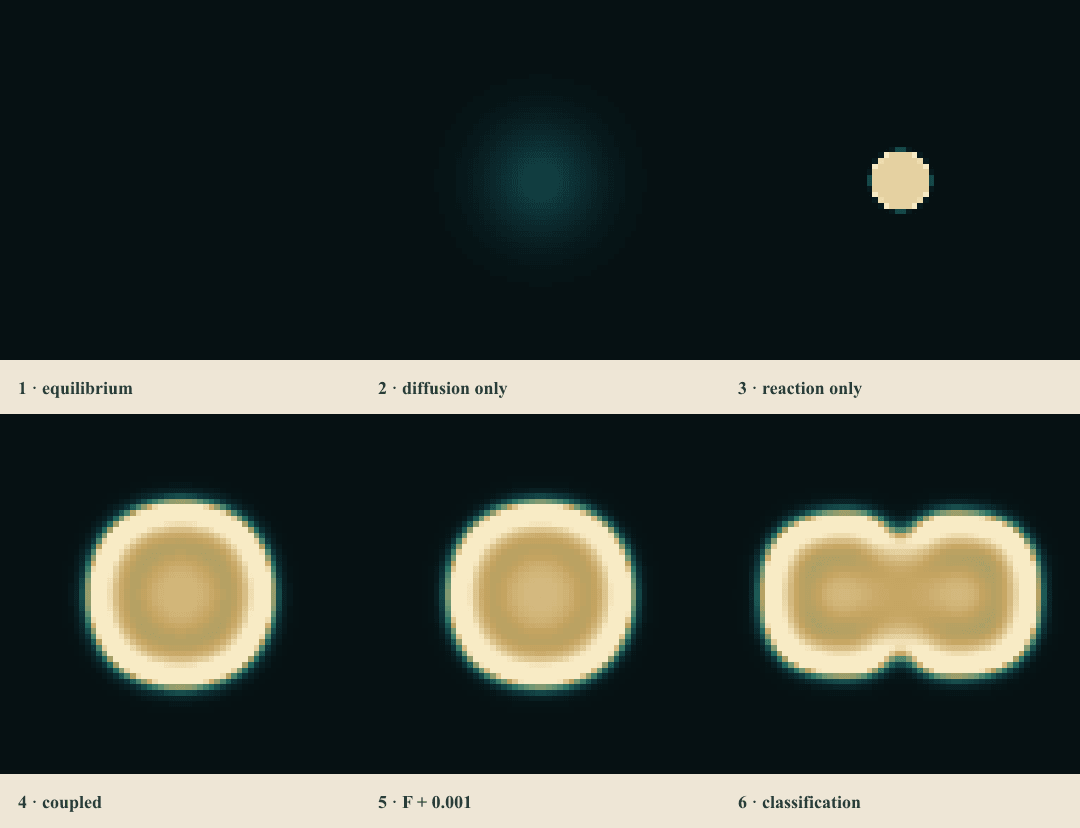
The first guided plate separates these claims. Deposit one patch, watch its variance fall, and compare its mean under periodic and no-flux walls. Then change only the boundary. The concentration is no longer obeying a vague tendency to blur; it is obeying a transport experiment whose domain is part of the method.

Guided observation · six controlled experiments

Six things to notice before touching every knob

Each plate starts from a declared field, advances a fixed-step Heun calculation, and can be replayed exactly. Nothing here is a video loop.

CPU reference 72 × 72 Δt 0.5 · periodic

UV

0%

step 0 / 48 model time 0.0

initial var(v)

0

current var(v)

0

active terms

4

Observation 1 of 6

The perfectly uneventful world

A control before the experiment

Look for

If every location begins at the feed state, where could a spatial feature come from?

Nowhere. At u = 1 and v = 0, diffusion sees no gradients and every reaction term is exactly zero. The replay advances the same integrator used below; the uniform field is a result, not a frozen illustration.

Active equation

u(x,y,0) = 1, v(x,y,0) = 0∂ₜu = 0, ∂ₜv = 0

diffusionautocatalysisfeedremoval

↳

Visible state. A uniform dark-green square remains uniform from edge to edge. No peak, front, or wavelength appears.

Preparing the deterministic initial field.

2. Chemistry that feeds upon itself

Now let two fields, $u$ and $v$, react locally. The Gray–Scott scheme is often summarized by the autocatalytic step

One unit of U is converted into V in the presence of two units of V. The existing V helps produce more V, which is why the step is called autocatalytic. In a mass-action model its rate is proportional to $uv^2$. Where either field is absent, that reaction stops. Where enough V already exists, the nonlinear square makes its influence rise quickly.

A closed tray would gradually exhaust its ingredients or settle according to whatever conserved totals and reactions it possessed. The Gray–Scott model used here is open. U is continuously restored towards a reservoir concentration, while V is removed. This feed and drainage can maintain a system away from equilibrium long enough for persistent fronts and localized structures to exist.

The letters must not be promoted into substances they have not earned. In this exhibit, U and V are dimensionless concentration-like fields. F and k are dimensionless model rates under the declared scaling. We are not claiming that the pale pixels are ferrocyanide, iodate, sulphite, an animal pigment, or anything waiting in a cupboard. The model is a mechanism made inspectable, not a labelled bottle.

3. The Gray–Scott equations, term by term

The complete model is

Every sign has a job.

• $D_u\nabla^2u$ and $D_v\nabla^2v$ transport each field according to its own diffusion coefficient.
• $-uv^2$ consumes U through the autocatalytic reaction.
• $+uv^2$ produces V at exactly the same local reaction rate.
• $F(1-u)$ restores U towards the reservoir value $u=1$.
• $-Fv$ removes V through the same open-system turnover associated with feed.
• $-kv$ supplies the additional kill or removal term.

The word kill is historical model vocabulary, not a tiny funeral. Nothing living is being killed. It is a first-order loss rate for V.

The matched $-uv^2$ and $+uv^2$ terms mean that the conversion itself transfers amount between the two fields. Add the two equations and those reaction terms cancel. The feed and removal terms do not cancel, however, so total $u+v$ is not conserved. Nor does diffusion guarantee a zero global contribution under every boundary: periodic and no-flux domains cancel internal fluxes in the sum, while a fixed reservoir can exchange with the domain.

This term-by-term ledger is more useful than assigning a zoological nickname to a finished texture. A labyrinth may be expanding because autocatalytic production is concentrated along its edge, while diffusion supplies U from outside and drains V across that edge. The visible form is the integrated history of those local balances.

4. A disturbance enters the room

The simplest homogeneous state is

It is the feed state: U is full, V is absent, the reaction rate $uv^2$ is zero, and every spatial derivative vanishes. Leave an exact numerical field there and it remains there. The machine is not embarrassed; a perfectly homogeneous initial condition has given it no reason to draw.

Pattern experiments therefore need a disturbance. The atlas can place a disk, ring, line, paired spots, seeded noise, or a recorded brush intervention. These are not interchangeable decorations. Infinitesimal noise asks whether arbitrarily small modes grow. A finite disk may cross a nonlinear threshold even when all infinitesimal modes around the equilibrium decay. A ring supplies more interface than a disk. Removing the original seed later asks whether the propagated structure has become dynamically self-sustaining elsewhere.

The distinction between infinitesimal and finite disturbances is the hinge between textbook linear instability and much of the Gray–Scott gallery. If an exact feed state stays quiet, that is not evidence that the implementation is broken. If a finite patch creates a persistent structure, that alone is not evidence that the feed state suffered a Turing instability.

The main observatory keeps model time separate from display time. It advances with a fixed numerical timestep, records interventions at simulation steps, and can run synchronized counterfactuals. Paint only into experiment A, hold the seed and parameters fixed in B, and the difference field reports the consequence of that intervention rather than the accident of two unsynchronized animation loops.

Gray–Scott model · fixed-step scientific instrument

Reaction–Diffusion Observatory

Two dimensionless concentration fields evolve from explicit equations. Display colour never changes the physics, and failed raw states are never made pretty by clamping.

experimentGS–H2–01schema 1 · five-point Laplacian

UV

64 model units

Preparing the scientific engine.

The stability number is 0.02000.

Run Reset Single step Step ×10 Replay in CPU reference Undo last intervention

Keyboard controls

With the field focused: Space runs or pauses; R resets; . steps once; arrow keys move the selected cell; Enter applies once; [ and ] change brush radius; 1–4 select Add V, Add U, Mixed pulse, or Restore feed; Escape cancels an active stroke.

model time0.00

step0

enginepreparing

rate— step/s

mean V—

variance V—

Current run · 256² · h 1.00 · μ 0.0800

grid256 × 256

domain L256.0 model units

h1.0000

Δt0.50000

μ / state0.080000 · safe

boundaryperiodic

seedobservatory-2407

F / k0.03670 / 0.06490

Dᵤ / Dᵥ0.1600 / 0.0800

mean U—

mean uv²—

wavelengthnone

equilibrium classlinearly-stable

events0 / 2000

history0 retained · 0 dropped

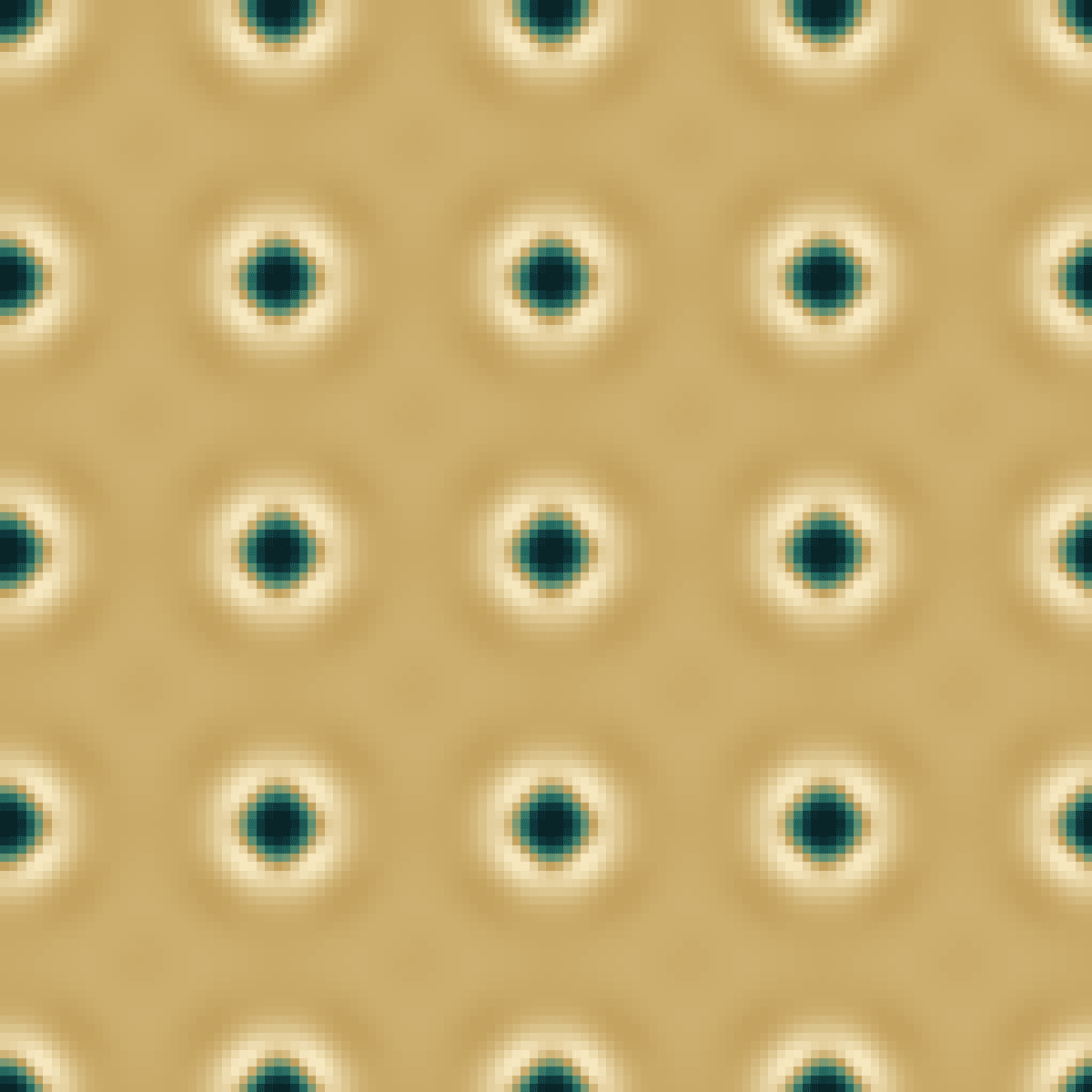
The field view comes first, but it is not the only witness. The current state includes its seed, grid, timestep, integrator, boundary, diffusion coefficients, F, k, model time, engine version, and ordered intervention log. A palette change belongs to display state and must not alter any of those concentrations.

5. The narrow geography of F and k

The feed rate F and kill rate k form a useful two-dimensional morphospace. Move horizontally and the rate at which U is restored and V is turned over changes. Move vertically and the additional loss of V changes. In a narrow region, a small move can separate a quiet decay from travelling fronts, repeated spot division, fluctuating filaments, or a field that fills and then collapses.

It is tempting to publish that plane as a butterfly collection: one tile labelled “worms”, another “mitosis”, another “coral”. The labels hide the experimental conditions. A tile is not the eternal phenotype of an $(F,k)$ coordinate. It is one finite-time field produced from a particular initial condition, domain, diffusion ratio, boundary, grid, timestep, and observation time.

That warning changed the instrument itself. Six candidate setups were rerun for 2,000 exact Float64 Heun steps on their declared $256\times256$ grids, all at the common model time $t=1000$. Three folklore-style names failed: their finite disturbances had already extinguished. The menu now says Collapse to feed state, Sparse-seed extinction, and Channel extinction where a decorative gallery might have promised dividing spots, worms, or selection. The surviving fields were named just as narrowly: Concentric vessel fronts, Seam-spanning bands, and Boundary-fed loop lattice. The adjacent machine-readable calibration record stores every setup, metric, spectrum verdict, engine version, step, model time, and field checksum.

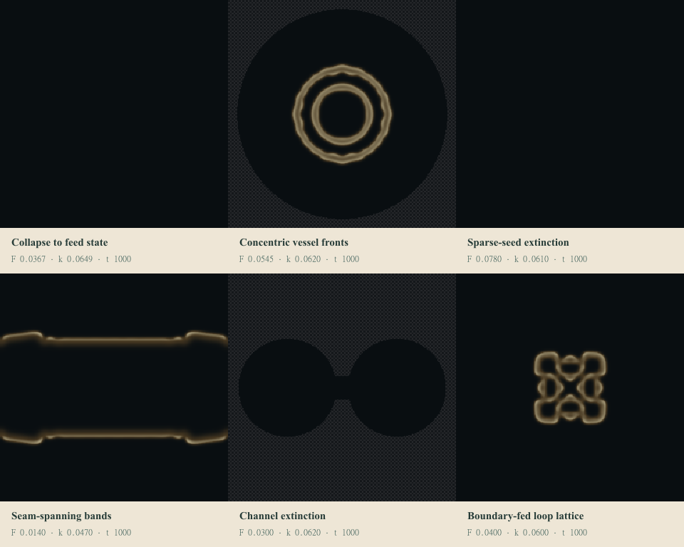
The named presets at their shared calibration checkpoint. Dark fields are measured extinctions, not missing images. Each label is conditional on the setup recorded beside the image and in the JSON evidence.

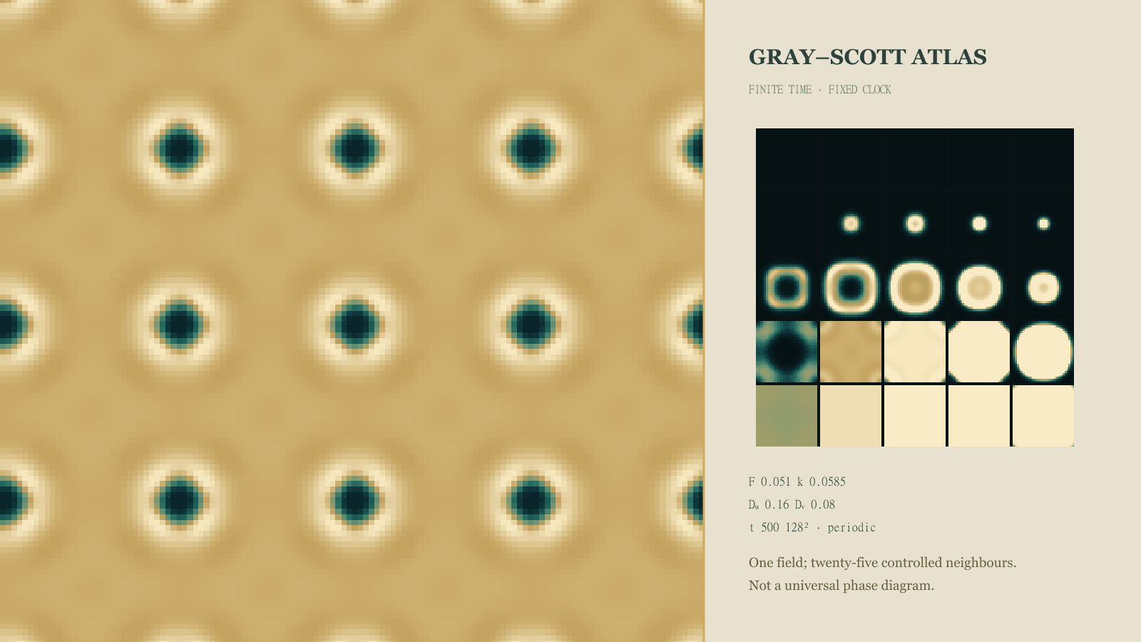
The morphospace below computes many small experiments under common controlled conditions. Each tile begins from the same declared seed and disturbance, advances to the same model time, and reports a compact measurement rather than a hand-selected picture. Click a tile to load its exact setup into the main observatory. Let it run longer and its description may change, because transient spots can split, merge, invade, or disappear.

Many controlled runs · one finite time

Feed–kill morphospace

This is a live finite-time morphospace under the displayed experiment—not a universal Gray–Scott phase diagram. Each square is an independent calculation.

Calculate atlas Pause

Atlas range and common observation time

F minimum F maximum k minimum k maximum Model time

Ready to calculate. The atlas does no work until you ask. 0%

Ready to calculate. The atlas does no work until you ask.

Calculation is intentionally idle. Choose a range if needed, then calculate the atlas.

Common conditions: D_U 0.16, D_V 0.08, Δt 0.5, periodic 32 × 32 grid, central soft disk, seed “observatory-2407”. Tile edges never exchange neighbours. Results depend on all of these choices and elapsed time.

Read adjacent tiles as controlled changes. A horizontal step changes F while preserving k; a vertical step changes k while preserving F. A diagonal jump changes both and cannot tell you which was responsible. The map is most useful as an experimental queue, not as an oracle.

6. Turing pattern, or merely a pattern people call Turing?

In 1952, Alan Turing asked how interacting, diffusing substances could help a homogeneous biological system develop spatial structure. His paper, “The Chemical Basis of Morphogenesis”, established a striking possibility: a reaction equilibrium that is stable to spatially uniform disturbances can become unstable to disturbances with non-zero spatial wavelength when diffusion is included.

That statement contains a test.

First find a homogeneous equilibrium $(u_*,v_*)$. Ignore diffusion and linearize the reaction terms around it. For the Gray–Scott kinetics, the reaction Jacobian is

If every eigenvalue of $J$ has negative real part, a small spatially uniform disturbance decays. Then examine a Fourier mode with wave number $q$. Diffusion changes the linear operator to

A classical stationary diffusion-driven instability requires stability at $q=0$ and positive growth for a band with $q>0$. If the uniform mode is already unstable, diffusion did not destabilize an otherwise stable equilibrium. If all scanned modes decay but a finite seed produces a pattern, the structure is nonlinear and finite-amplitude rather than a linear Turing instability of that equilibrium.

At the feed state $(1,0)$, the reaction Jacobian is diagonal with entries $-F$ and $-(F+k)$. For positive rates it is linearly stable, and adding ordinary positive diffusion makes the diagonal contributions more negative for non-zero modes. The familiar seeded Gray–Scott structures therefore do not become textbook Turing instabilities of the feed equilibrium merely because they are spotted.

The model can also possess two non-trivial homogeneous equilibria when

Their U coordinates are

with $v_*=(F+k)/u_*$. Those equilibria have their own reaction stability and diffusion-modified spectra. The inspector calculates them when the discriminant permits, rather than conjuring a non-trivial equilibrium for every preset.

Reaction Jacobian · spatial modes

Homogeneous equilibrium and stability inspector

The classification asks a strict question: is a homogeneous reaction equilibrium stable at q = 0 yet unstable after diffusion modifies at least one non-zero spatial mode?

Linearly stable over the scanned modes

This run needs more than an infinitesimal perturbation around this tested equilibrium; a finite disturbance and nonlinear trajectory can still make structure.

The zero line separates decaying modes below from growing modes above. The scan extends across the displayed resolvable range.

Equilibrium (u*, v*)

(1.0000, 0.0000)

trace J

-0.13830

det J

0.0037287

λ₁(0)

-0.03670

λ₂(0)

-0.1016

max growth

-0.036700

fastest q

none

linear wavelength

not meaningful

Dispersion values as a table

Representative samples from max Re λ(q)

q	Maximum real growth rate	Mode
0.0000	-0.036700	decaying
0.24544	-0.046338	decaying
0.49087	-0.075253	decaying
0.73631	-0.12344	decaying
0.98175	-0.17871	decaying
1.2272	-0.22208	decaying
1.4726	-0.27509	decaying
1.7181	-0.33774	decaying
1.9635	-0.41003	decaying
2.2089	-0.49195	decaying
2.4544	-0.58351	decaying
2.6998	-0.68472	decaying
2.9452	-0.79556	decaying

The classification panel reports the equilibrium examined, the reaction eigenvalues at $q=0$, the fastest scanned spatial mode, and the conditions used for its verdict. “Finite-amplitude nonlinear structure” is not a demotion. Nonlinear localized states, fronts, excitability, and multistability are scientifically rich. The purpose is to name the mechanism being tested instead of using Turing’s surname as a compliment for any attractive stripe.

John Pearson’s 1993 paper “Complex Patterns in a Simple System” documented a remarkable finite-amplitude Gray–Scott pattern catalogue. It is a central source for this atlas precisely because its nonlinear structures should be studied on their own terms. Mark Cross and Pierre Hohenberg’s broad review of pattern formation outside equilibrium supplies the larger framework: thresholds, modes, nonlinear regimes, boundaries, defects, and the difference between an onset calculation and a developed pattern.

7. What is happening at one pixel?

A field image compresses thousands of local ledgers into colour. Select one cell and the microscope opens those ledgers.

For U it reports diffusion import or export, reaction consumption, feed restoration, their total right-hand side, and the observed change after the integrator step. For V it reports diffusion, reaction production, feed-related removal, additional kill, total right-hand side, and observed change. Signed bars use a zero-centred scale and explicit plus and minus labels; colour is never the only indication of direction.

The discrete five-point Laplacian at an interior grid cell is approximately

The same stencil is applied to V. It does not inspect an abstract smooth surface; it inspects four numerical neighbours separated by grid spacing $h$. Periodic edges wrap those neighbour lookups. No-flux edges replace outward exchange with a reflected value. An impermeable obstacle removes transport across the masked face. A reservoir edge supplies its fixed state. Boundary code is therefore part of the equation actually solved.

One cell · every term

Reaction–diffusion microscope

Cell (0, 0) contains u = 1.0000 and v = 0.0000. Values below are dimensionless concentration change per model-time unit.

N0.000

W0.000

V centre0.000

E0.000

S0.000

∇²v = 0

U ledger

diffusion

0

−uv²

0

feed

0

Net ∂u/∂t

0

V ledger

diffusion

0

+uv²

0

feed removal

0

kill

0

Net ∂v/∂t

0

Recent selected-cell record

Local concentration history

0 samples

Run or step the laboratory to collect a bounded u/v trace for this cell.

Reaction-only kinetics · spatial overlay

Local phase plane

u–v state space

The nullclines describe a spatially isolated cell. Diffusion is overlaid at the selected cell from its four actual neighbours; it is not a function of (u, v) alone.

f(u,v) = −uv² + F(1−u) = 0 g(u,v) = uv² − (F+k)v = 0

f=0g=0equilibriumreaction onlyactual diffusionnet

Arrows use a common tangent horizon τ = 20.0 model-time units to make direction legible; they are derivatives at this instant, not integrated trajectories.

Vectors at selected (u, v)

Vector	du/dt	dv/dt	Depends on
Reaction only	0	0	selected u, v; F, k
Actual diffusion	0	0	north, south, east, west; Dᵤ, Dᵥ; boundary
Net PDE	0	0	reaction + actual diffusion

Exact local PDE ledger

Field	Diffusion	Autocatalysis	Feed	Kill	Total
U	0	0	0	—	0
V	0	0	0	0	0

The global budget averages the same terms across all active cells:

For periodic and correctly implemented no-flux boundaries, the integrated diffusion contribution should be approximately zero: internal transfers cancel in pairs. That does not mean diffusion is locally inactive. A growing edge can receive V by reaction at one cell, lose it by diffusion there, and deliver it to the next cell while the domain-wide diffusion sum remains near zero.

The budget also compares the right-hand-side prediction with the measured mean change. A persistent discrepancy is not decorative uncertainty; it is a reason to inspect event timing, masks, boundary flux, or the integrator.

8. Walls are part of the experiment

A periodic square has no ordinary wall. A front crossing its right edge enters from the left and may collide with itself. A no-flux square has impermeable walls: concentration may accumulate beside them, fronts meet them, and normal transport vanishes. A feed-reservoir wall continually imposes $u=1$, $v=0$ at the edge, which can extinguish V nearby or supply U to a hungry front.

Geometry adds more questions. A narrow channel selects which structures fit through it. A circular obstacle bends an advancing front and creates a wake. Two openings can split a wave and make its branches collide. An impermeable island is not merely black paint over the rendered field; the stencil must prevent chemical flux through the mask.

This is why changing a boundary is not a display option. It changes the mathematical experiment. Compare mode can hold F, k, seed, grid, timestep, and intervention history fixed while changing only the boundary. The difference map then has an intelligible counterfactual meaning.

Try placing a spot near a periodic seam and then near a no-flux wall. In the first case its “neighbour” may be on the far side of the image. In the second, the wall removes that route. The eventual difference can fill the domain even though the initial edit occupied only a few cells.

9. Measuring pattern rather than admiring it

The domain mean says how much U or V is present on average. Variance says how strongly the field differs across space. Neither identifies a characteristic spacing. For that, the atlas examines spatial frequency.

The spectrum begins by subtracting the mean, because the average concentration is a zero-frequency component rather than a pattern wavelength. An optional stated window reduces the artificial seam created by treating a non-periodic crop as periodic. A two-dimensional Fourier transform distributes power across horizontal and vertical wave vectors. Radial averaging then groups power by the magnitude of the wave vector, producing a one-dimensional spectrum.

If a credible non-zero peak occurs at spatial frequency $f_*$, the corresponding wavelength is approximately

The units are dimensionless model length, not pixels, provided grid spacing and domain length are accounted for. A finer grid over the same domain should not halve the reported physical wavelength simply because it contains twice as many cells.

FFT · radial average · measured scale

Spatial spectrum and dominant wavelength

The field mean is removed first. No window is applied to this periodic field.

No invented peak none

measured field

not yet measured

q*

—

domain fraction

—

peak prominence

0.00

window

none

No trustworthy dominant wavelength is present: the field has no resolved variation.

Spectrum values as a table

Radially averaged power by wave-number bin

q	Power
0.0000	0.0000
0.025000	0.0000
0.050000	0.0000
0.075000	0.0000
0.10000	0.0000
0.12500	0.0000
0.15000	0.0000
0.17500	0.0000
0.20000	0.0000
0.22500	0.0000
0.25000	0.0000
0.27500	0.0000
0.30000	0.0000
0.32500	0.0000
0.35000	0.0000
0.37500	0.0000
0.40000	0.0000
0.42500	0.0000
0.45000	0.0000
0.47500	0.0000
0.50000	0.0000
0.52500	0.0000
0.55000	0.0000
0.57500	0.0000
0.60000	0.0000
0.62500	0.0000
0.65000	0.0000
0.67500	0.0000
0.70000	0.0000
0.72500	0.0000
0.75000	0.0000
0.77500	0.0000
0.80000	0.0000

Radial averaging is useful and lossy. It treats every direction alike. Parallel stripes can have a sharp directional spectrum whose radial summary conceals orientation. A single travelling front, one isolated spot, or a strongly non-stationary mixture may have no honest dominant wavelength. In those cases the instrument says that no trustworthy peak was found and exposes the spectrum and table rather than awarding a number to keep the panel occupied.

A spectral peak also does not prove a Turing mechanism. Linear stability predicts which infinitesimal modes grow near a specified equilibrium. A Fourier spectrum measures structure in a finite nonlinear field at a specified time. Agreement can be informative; disagreement can be more informative; neither plot is a substitute for the other.

10. Spots that divide, without becoming organisms

Some Gray–Scott settings produce localized V-rich spots that widen, deform into a dumbbell, pinch, and leave two spots. Repetition can populate a field with descendants of the original concentration patch. Pearson’s simulations made such structures prominent, and Kyoung-Jin Lee, William McCormick, Pearson, and Harry Swinney later reported experimental self-replicating spots in a ferrocyanide–iodate–sulphite reaction–diffusion system.

The experimental result matters. It shows that repeated spot growth and division are not confined to a screen. It does not make every numerical Gray–Scott spot a reconstruction of that chemical experiment, and it does not turn geometric replication into life.

Here self-replicating has a narrow operational meaning: a localized concentration structure produces additional localized structures through the declared reaction–diffusion dynamics. There is no membrane maintaining an internal physiology, no genome, no copying of hereditary information, no metabolism, no adaptation, and no lineage exposed to natural selection. The offspring metaphor is convenient for counting spots and treacherous if allowed to carry biological luggage.

Shigeru Kondo and Takashi Miura review the reaction–diffusion framework in biological pattern formation with examples in which theory and experiment can inform one another. That is the appropriate standard. Visual resemblance can suggest a mechanism to test. Establishing that mechanism in a tissue requires identifying relevant molecules, interactions, transport, geometry, perturbation responses, and competing explanations.

11. The calculation can counterfeit the chemistry

The equations are continuous. The browser stores a finite grid and advances it by finite timesteps. Between those statements lies the possibility of numerical fraud committed without malice.

For a two-dimensional five-point diffusion stencil advanced by explicit Euler, a familiar necessary diffusion bound is

It is not a complete guarantee for the coupled nonlinear reaction system. Strong local reaction can require a smaller step, and boundaries or implementation details can add constraints. Heun’s method evaluates a predictor and a correction and has second-order accuracy on smooth problems, but it remains explicit and does not repeal stability limits.

The atlas detects non-finite values, implausible growth, and declared stability violations. It does not silently clamp concentrations into the unit interval from zero to one and continue the film. Clamping can hide the first evidence of an unsafe timestep, alter conservation and budgets, and manufacture an apparently stable attractor. If the state becomes unsafe, the run stops with the reason and last valid record available.

Convergence · stability · no quiet repairs

Is the pattern in the equation, or in the calculation?

Visual resemblance, numerical convergence and physical validity are three separate claims. These controlled pairs test the first two; neither can validate the idealised model against nature.

Preparing the dedicated numerical-comparison Worker.

Δt versus Δt/2

Does halving the step change the field at equal model time?

Same domain, field, boundary and Heun method; only the fixed timestep changes.

Run comparison

No calculation has been run in this session.

Coarse versus fine h

Does the morphology survive a smaller grid spacing?

Same physical domain and continuous seed, resampled on two stable grids.

Run comparison

No calculation has been run in this session.

Euler versus Heun

How much does integration order matter over a controlled interval?

Both methods meet a smaller-step Heun reference at the same model time.

Run comparison

No calculation has been run in this session.

Deliberately unsafe Δt

What does numerical failure look like without a clipping rescue?

Opt-in run above the explicit diffusion ceiling; pause at the first invalid state.

Run comparison

No calculation has been run in this session.

The laboratory compares Euler with Heun at equal model time, not equal frame count. It can repeat a controlled run at $\Delta t$ and $\Delta t/2$, and compare grids representing the same physical domain rather than unrelated arrays. A visually small difference is quantified by field norms and summary metrics. A visually dramatic difference is not automatically evidence that the finer run is correct; convergence requires a sequence approaching a stable answer.

Floating-point reproducibility has limits too. The deterministic CPU engine is the reference implementation and can replay the same initial arrays and ordered interventions. The GPU uses the same documented equations and boundary semantics, but shader arithmetic may differ in evaluation order and precision across hardware. Agreement within a documented tolerance over a short controlled run is meaningful. Cross-device bitwise identity is not promised.

A stable movie is a weak test. A trustworthy calculation also needs expected invariants: the feed equilibrium remains fixed; constant fields have zero Laplacian; pure periodic or no-flux diffusion conserves the mean and reduces variance; reaction-only cells do not communicate; integrated diffusion nearly cancels where it should; measured mean change reconciles with the budget; and refinement changes the result in the expected direction.

12. Experiments worth trying

Each of these investigations changes one declared part of the experiment and asks for an observable result.

1. Hold F and k fixed and change only the boundary. Compare periodic, no-flux, and feed-reservoir runs at equal model time. Identify where their difference field first becomes non-zero.
2. Compare a disk with a ring disturbance. Give them similar total V, then ask whether the extra interface in the ring changes the onset time or number of surviving spots.
3. Find a finite-amplitude pattern around a linearly stable feed state. Confirm that the stability inspector finds no growing infinitesimal mode there, then reduce the seed amplitude until the structure no longer survives.
4. Halve $D_v$ while preserving every other value. Measure the dominant wavelength only if the spectrum reports a credible peak; state whether the change agrees with your qualitative expectation.
5. Walk one morphospace tile horizontally, then vertically. Keep the common initial condition and observation time. Decide whether changing F or k had the larger measured effect in that neighbourhood.
6. Repeat one run at $\Delta t$ and $\Delta t/2$. Compare at equal model time using both a field norm and the global budget discrepancy.
7. Build a narrow channel. Observe which fronts pass, which become oriented, and whether widening the channel produces a threshold rather than a smooth visual change.
8. Remove the original spot after the pattern has spread. Record the intervention step and test whether distant structures persist without confusing persistence with biological autonomy.
9. Apply the same brush intervention to A only in Compare mode. Follow the difference map and mean absolute field difference while both runs advance through the same fixed timesteps.
10. Find a field with no credible spectral peak. Explain why the “no peak” result is more accurate than reporting the tallest noisy bin as a wavelength.

13. What this model does not establish

The Gray–Scott atlas is a two-field idealized partial differential equation. Its U and V values are dimensionless fields. Unless a specific experiment deliberately adds it, there is no molecular noise. There is no fluid flow, temperature field, mechanical deformation, or growth of the domain.

There is no gene regulation. There are no cells. There is no metabolism, membrane, heredity, adaptation, natural selection, perception, purpose, or struggle for existence. A spot that splits is a concentration structure changing topology.

The selected F, k, $D_u$, and $D_v$ values are not measurements of an animal skin. The model demonstrates a mechanism class, not a universal explanation of biological form. A plausible resemblance can motivate a biological experiment; it cannot replace one.

Numerical agreement across resolutions increases confidence that the discrete calculation is approximating the declared equations. It does not validate those equations against nature. Conversely, disagreement between resolutions is a warning about the calculation before any biological interpretation begins.

The atlas also omits many mechanisms that create pattern: advection, phase separation, mechanics, differential growth, cell movement, stochastic nucleation, pre-existing geometry, external gradients, and networks with more than two interacting species. Reaction–diffusion is a powerful sentence in the language of pattern formation, not the whole dictionary.

For neighbouring instruments, the Brownian Motion Laboratory isolates diffusion and stochastic motion; the Artificial Life Lab includes inheritance and selection that this model explicitly lacks; the Double-Pendulum Atlas separates deterministic sensitivity from numerical error; and Gradient Descent Landscapes asks how a local update rule navigates a larger state space.

Sources and further reading

• Alan M. Turing, “The Chemical Basis of Morphogenesis”, Philosophical Transactions of the Royal Society of London. Series B, 1952. The original linear reaction–diffusion morphogenesis argument.
• John E. Pearson, “Complex Patterns in a Simple System”, Science, 1993. The foundational finite-amplitude Gray–Scott pattern catalogue.
• K. J. Lee, W. D. McCormick, J. E. Pearson, and H. L. Swinney, “Experimental Observation of Self-Replicating Spots in a Reaction–Diffusion System”, Nature, 1994. Laboratory observation of repeated spot growth and replication.
• Michael C. Cross and Pierre C. Hohenberg, “Pattern Formation Outside of Equilibrium”, Reviews of Modern Physics, 1993. A wider framework for onset, modes, nonlinear patterns, boundaries, and defects.
• Shigeru Kondo and Takashi Miura, “Reaction-Diffusion Model as a Framework for Understanding Biological Pattern Formation”, Science, 2010. A cautious modern review of reaction–diffusion reasoning in biology.

Choose one morphospace tile that produces spots at the published observation time. Load it into the observatory, halve the timestep, keep the seed and boundary fixed, and run both calculations to the same model time. The next useful fact is whether the spots survive that comparison.