The Particle That Could Not Make Up Its Mind

A Brownian Motion Laboratory

The particle is already moving. It has been given no destination, no memory and no talent for looking decisive. Every fraction of a second it accepts another microscopic kick and revises its opinion about where to go. Watched alone, it appears to be doing nothing in particular.

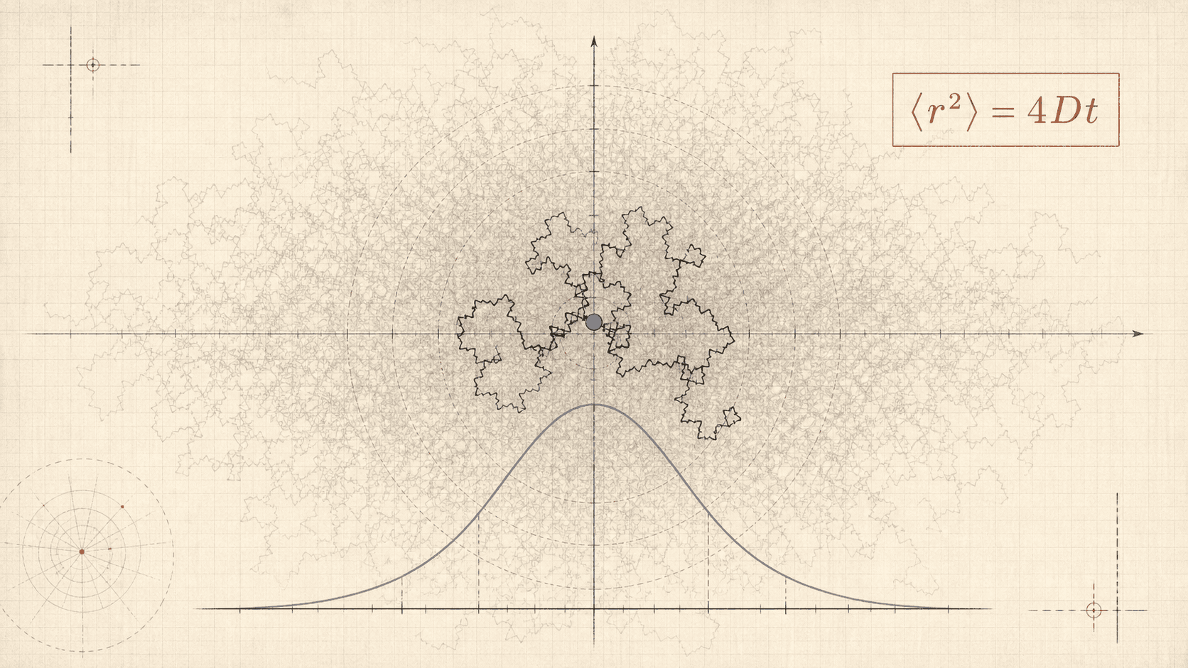
Make nine hundred and ninety-nine copies, however, and the insult to intuition becomes more interesting. The individual lines remain unruly. The crowd becomes a smooth cloud. Its centre, width and entire probability distribution begin obeying equations with unnerving punctuality.

Audio article

Uses the speech voice supplied by your browser or device.

Begin here: let the first particle run for a moment. Pause it, press Reset and confirm that the same seed redraws the same path. Then choose Add more particles until the density and mean-square-displacement views appear. The short note beneath each process says what to watch; the advanced controls can wait.

A Brownian Motion Laboratory · browser-local · deterministic

The Particle That Could Not Make Up Its Mind

One path is gossip. A crowd keeps accounts.

simulated time 0.000 s fixed Δt 0.00833

Pause Reset New seed

A Brownian-motion stage. The text status and measurement table below report the same experiment numerically.

drag to pan · Ctrl/⌘ + wheel to zoom · arrows / + / − / 0

One particle looks confused. Add 999 more.Add independent copies to reveal the distribution and its law.

Add 999 more particles

Calibrating independent random streams.

Solid marks are measurements from this run. Dashed marks are theoretical predictions. A translucent band is a stated variance or uncertainty interval, never decorative fog.

1. One particle tells a terrible story

A trajectory is an anecdote: vivid, memorable and statistically weak. A long excursion to the right may look like a preference. A tight knot may look like confinement. Neither conclusion is justified until the same rule has been repeated across many independent histories or across many time origins.

Start with a humbler object than Brownian motion: a discrete random walk. Suppose a walker takes a step of length $\ell$ every $\tau$ seconds, choosing symmetrically among directions in $d$ dimensions. Its large-scale diffusion coefficient is

In plain language, smaller steps do not necessarily mean slower large-scale spreading. If we shorten the waiting time at the same rate as we shrink the squared step length, $D$ stays fixed.

After $n$ independent, unbiased steps, the cross terms cancel on average and the squared displacement grows in proportion to $n$. Since $t=n\tau$,

In plain language, a typical distance grows like the square root of the number of steps even though the squared distance grows like the number of steps itself.

Try Discrete random walk → Shrink the steps. The blocky path gains more, smaller corners while the broad cloud changes very little. This is a scaling-limit story: suitably rescaled random walks converge in distribution to Brownian motion. It is not a claim that an ideal Brownian path is secretly a finite lattice walk seen from far away.

The central mode uses the overdamped Brownian update independently in the two visible directions:

where $D$ is the diffusion coefficient, $\Delta t$ is one fixed physical timestep, and $\xi_x$ and $\xi_y$ are independent standard normal values. In plain language, the kick grows with the square root of elapsed time. Wait four times as long and a typical displacement becomes roughly twice as large, not four times as large.

The same law is often written more compactly as

In plain language, $d\mathbf{W}$ denotes an ideal Gaussian increment whose variance is proportional to time; it does not mean that an ordinary, finite velocity is being multiplied by a tiny time interval.

The browser draws whenever the display is ready, but the model advances only in fixed increments. A 30 Hz screen and a 120 Hz screen therefore consume the same random values after the same number of physics steps. Pausing, adding an analytical circle or changing a particle’s display size does not secretly change its future.

2. The crowd becomes a bell curve

Independent kicks add. Their positive and negative parts mostly cancel in the mean, while their variances accumulate. For one coordinate of a freely diffusing particle that began at the origin,

In plain language, doubling the elapsed time doubles the horizontal spread measured as a variance. It does not double the ordinary width; the standard deviation grows only by $\sqrt{2}$.

The horizontal and vertical coordinates follow the same rule independently. For a particle released at $\mathbf{x}_0$, their joint distribution is a circular two-dimensional Gaussian:

In plain language, no particular destination is favoured, yet positions near the release point remain more probable than equally sized patches far away. The dashed circles in the stage use the selected $D$ and the very same simulated time that advances the particles.

The one-coordinate distribution tab shows the corresponding bell curve,

In plain language, the area under the curve stays one while the curve becomes lower and wider. Probability is spreading, not disappearing.

A bead in water, with the assumptions left visible

The Colloidal bead in water preset gives the symbols physical units through the Stokes–Einstein relation:

In plain language, a warmer fluid increases diffusion, while a more viscous fluid or a larger spherical bead reduces it. Under the preset values—$T=298.15\ \mathrm{K}$, water viscosity $\eta=0.89\ \mathrm{mPa\,s}$ and bead radius $a=0.50\ \mu\mathrm{m}$—the estimate is about $0.49\ \mu\mathrm{m}^2\mathrm{/s}$.

That number comes with conditions. The bead is assumed spherical; the flow has very low Reynolds number; the liquid is treated as a continuum; the suspension is dilute and noninteracting; thermal equilibrium holds; and there is no nearby-wall correction. The moving dot is an effective Langevin description of many molecular encounters. Any visible “molecular kicks” are schematic, not a count or scale model of water molecules striking the bead.

A compact history, without retrospective mythology. In observations made from June to August 1827, Robert Brown studied moving microscopic particles associated with pollen and then found similar motion in inert material; his 1828 account did not reveal molecules and did not show that pollen was alive. Albert Einstein’s 1905 paper gave a statistical connection between diffusion and molecular motion. Marian Smoluchowski developed a related treatment independently, published in 1906. Jean Perrin’s painstaking measurements, reported in his 1909 study and later reviewed in his Nobel lecture, became important cumulative evidence for the molecular view of matter—not a single magical proof. Paul Langevin’s 1908 note recast the problem as a balance between drag and a fluctuating force. It is best read as a physical force argument, not as today’s fully rigorous white-noise formalism. The 1930 paper by George Uhlenbeck and Leonard Ornstein treated velocity relaxation, the idea restored in this laboratory’s underdamped mode.

3. Why the mean-square displacement matters

Average displacement is a poor witness for unbiased diffusion. Left and right cancel; up and down cancel. Squaring removes the sign while keeping the size of each excursion. For $N$ particles in two dimensions the measured radial mean-square displacement is

In plain language, the laboratory measures how far every particle has travelled from its own starting point, squares those distances and then averages them. A path that goes left is no longer allowed to cancel a path that goes right.

Each coordinate contributes $2Dt$, so the two-dimensional prediction is

In plain language, distance itself grows on the scale of $\sqrt{t}$ while squared distance grows linearly with $t$. The factor four is not universal: it is $2d$ in $d$ spatial dimensions under this convention for $D$.

The graph deliberately keeps the noisy measured line and the smooth theoretical line distinct. Agreement means statistical closeness over an adequate ensemble, not pixel-perfect overlap. With one particle the curve can wander extravagantly; with thousands, its sampling fluctuations usually shrink. A standard-error band, when shown, is calculated from the ensemble rather than painted in for reassurance.

Show derivation: why independent steps produce MSD proportional to time

Write a one-dimensional displacement after $n$ steps as

$$X_n-X_0=\sum_{j=1}^{n}\delta X_j.$$

In plain language, the final displacement is simply the sum of all microscopic displacements.

Squaring and averaging gives diagonal terms plus cross terms:

$$\mathbb{E}\bigl((X_n-X_0)^2\bigr) =\sum_{j=1}^{n}\mathbb{E}(\delta X_j^2) +2\sum_{j<k}\mathbb{E}(\delta X_j\delta X_k).$$

In plain language, the first sum records the size of every step; the second asks whether the sign of one step predicts another.

For independent zero-mean increments, each cross expectation is zero. If each step has variance $\sigma^2$, then

$$\mathbb{E}\bigl((X_n-X_0)^2\bigr)=n\sigma^2.$$

In plain language, $n$ equally noisy, uncorrelated steps contribute $n$ equal pieces of variance. Since elapsed time is proportional to $n$, the MSD is proportional to time.

Show derivation: why free Brownian motion gives 4Dt in two dimensions

The two-dimensional squared displacement separates into its coordinate contributions:

$$|\mathbf{X}(t)-\mathbf{X}(0)|^2 =(X(t)-X(0))^2+(Y(t)-Y(0))^2.$$

In plain language, Pythagoras turns radial squared distance into horizontal squared distance plus vertical squared distance.

Each independent coordinate has variance $2Dt$, so

$$\mathbb{E}\bigl(|\mathbf{X}(t)-\mathbf{X}(0)|^2\bigr)=2Dt+2Dt=4Dt.$$

In plain language, both visible dimensions contribute the same $2Dt$ to the total.

The local diffusion exponent asks for the slope of the MSD curve on logarithmic axes:

In plain language, $\alpha$ near one signals ordinary diffusive scaling over that interval, near two signals ballistic scaling, and other values may reveal confinement, correlations or a crossover. A short, noisy trace can imitate any of these, so the slope is a diagnostic rather than a verdict.

4. Randomness is not the absence of law

Brownian motion is a probability law over paths, not a claim that every squiggle means the same thing. At the ensemble level the free density obeys the diffusion equation

In plain language, probability flows away from locally concentrated regions. The equation predicts the evolving density, not the next turn of one chosen particle.

Direction can matter

In a narrow channel or layered material, spreading need not be circular. The anisotropic mode chooses two non-negative principal diffusion coefficients, $D_1$ and $D_2$, and rotates their axes by $\theta$:

In plain language, independent Gaussian kicks are stretched by different amounts along two material axes and then rotated into the screen coordinates. The circular cloud becomes an ellipse whose axes and widths are predicted by the diffusion tensor. The laboratory refuses negative coefficients because they would not define a valid covariance.

When the screen axes are not aligned with the principal axes, the displayed $x$ and $y$ increments can have nonzero covariance. That is spatial correlation within one step, not memory between different times.

The Isotropic versus anisotropic comparison can use matched Gaussian samples. Each side then receives corresponding random numbers, making the change in the material law easier to see. Matched noise is a teaching device, not a claim that two independent physical experiments would share microscopic kicks.

A boundary changes what can be inferred

Reflecting walls, periodic seams and absorbing walls answer different questions. A reflection preserves the particle but reverses the overshooting part of a step; merely clamping it to the wall would manufacture a false pile-up. A periodic stage wraps the drawn position, but the engine retains an unwrapped position for displacement statistics. Otherwise every seam crossing would look like an enormous jump backwards. An absorbing wall removes a particle when it first crosses and turns a location problem into an arrival-time problem.

Finite domains eventually alter the free-space law. A reflecting box reaches a stationary spatial distribution, so its radial MSD cannot grow as $4Dt$ forever. A periodic display can look stationary while its unwrapped displacement continues to grow. The theory overlay changes with the boundary rather than pretending the free Gaussian survives every intervention.

Put the randomness on a landscape

An overdamped particle in a potential $U$ follows

In plain language, the slope of the landscape pulls the particle downhill while thermal noise keeps kicking it away from deterministic descent. Mobility $\mu$ controls how readily it responds.

At equilibrium, the stationary density has the Boltzmann form

In plain language, low-potential regions are more heavily occupied, but a sufficiently warm particle can still cross a barrier. In the double-well preset, rare hops become common as the barrier is lowered or the temperature is raised. The harmonic, double-well, corrugated, tilted and obstacle landscapes are different models, not different colours for the same path.

A static asymmetric potential at thermal equilibrium does not generate a perpetual directed ratchet current. Directed ratchet motion requires explicit nonequilibrium driving, switching or another broken-detailed-balance mechanism. The laboratory labels any such drive rather than hiding it in an attractive asymmetric drawing.

Show derivation: why mobility and temperature determine diffusion

For one coordinate, the Fokker–Planck probability current associated with the landscape model is

$$J=-\mu U'(x)p-D\frac{\partial p}{\partial x}.$$

In plain language, one part of the probability current comes from deterministic downhill drift and the other from diffusive spreading.

At thermal equilibrium the current vanishes and $p$ is proportional to $\exp(-U/(k_{\mathrm B}T))$. Substitution gives

$$0=-\mu U'(x)p +\frac{D}{k_{\mathrm B}T}U'(x)p.$$

In plain language, equilibrium requires the downhill response and thermal broadening to balance at every ordinary point of the potential.

Therefore

$$D=\mu k_{\mathrm B}T.$$

In plain language, stronger mobility or higher temperature produces stronger diffusion. For a sphere with low-Reynolds-number mobility $\mu=(6\pi\eta a)^{-1}$, this becomes the Stokes–Einstein expression used by the physical preset.

5. Add a current

Random spreading and directed transport can occur simultaneously. With a constant drift velocity $\mathbf{v}$,

In plain language, every particle receives the same steady translation as well as its own independent random kick.

The centre of an ensemble released at $\mathbf{x}_0$ follows

In plain language, the cloud’s centre moves in a straight line at the imposed velocity.

Meanwhile each coordinate retains

In plain language, a constant current moves the bell curve without changing its diffusive width. Drag the vector arrow, then enable the co-moving frame: subtracting $\mathbf{v}t$ should make the cloud look like ordinary free diffusion again.

If the optional force view is used, velocity is written as $\mathbf{v}=\mu\mathbf{F}$. In plain language, the displayed force produces drift through a stated mobility; force and velocity are not silently treated as the same quantity.

Comparison guide: choose a paired preset, press Reset both, then toggle Matched noise where it is offered. Look first at the same time and camera scale; only then change one parameter. Solid curves are measured separately on each side.

A/B stochastic workbench

Same seed. Different physics.

Does a moving mean change the rate at which the cloud broadens?

Ensemble 52 × 2 129 points each

Comparison preset 01 · Free vs drift02 · Isotropic vs anisotropic03 · Overdamped vs underdamped04 · Passive vs active05 · Brownian vs fractional06 · Brownian vs Lévy07 · Weak vs strong trap08 · Low vs high temperature

Replay seed Apply Next seed

Camera

Linked Independent

Matched noise

Coupling: Both panels share every Gaussian kick; the right panel adds only μ dt.

Observation time

t = 4.00 s

A

Free Brownian

dX = √(2D) dW

＋ − Fit A

Mean x

measured+0.034

theory0.000

Radial MSD

measured5.122

theory6.400

σₓ / σᵧ

measured1.546 / 1.651

theory1.789 / 1.789

Theory. Exact Gaussian propagator; radial MSD = 4Dt.

•••

B

Drift–diffusion

dX = μ dt + √(2D) dW

＋ − Fit B

Mean x

measured+2.634

theory+2.600

Radial MSD

measured12.06

theory13.16

σₓ / σᵧ

measured1.546 / 1.651

theory1.789 / 1.789

Theory. The mean moves as μt; centred variance still grows as 4Dt.

Matched noise is available only when the two algorithms can consume equivalent Gaussian samples without changing their meaning. Brownian versus Lévy flight, for example, cannot be made “fair” by pretending their increments share one distribution.

6. Put the particle in a trap

Now attach an invisible spring to an equilibrium point $\mathbf{m}$. The overdamped Ornstein–Uhlenbeck model is

In plain language, the farther the particle strays, the stronger the average pull back; random kicks prevent it from settling perfectly at the centre. This is an ideal harmonic trap. It can approximate an optical trap near a stable point, but the drawing is not a claim to simulate a particular tweezer apparatus.

For one coordinate starting at $x_0$, the mean relaxes as

In plain language, the ensemble centre forgets its initial displacement over a relaxation time of order $1/\lambda$.

Starting from a precise point, its time-dependent variance is

In plain language, the cloud initially broadens but eventually stops widening because the restoring pull balances diffusion.

At stationarity,

In plain language, stronger noise makes a wider equilibrium cloud and a stronger trap makes a narrower one. Drag the trap centre while the run is active: the cloud should lag behind and then relax, rather than teleporting with the target.

For a stationary coordinate, the position autocovariance decays as

In plain language, confinement introduces a memory in position even though the driving increments themselves remain independent: nearby observations resemble one another because the spring relaxes gradually.

Show derivation: the Ornstein–Uhlenbeck stationary variance

The exact solution separates the decayed starting point from accumulated noise:

$$X(t)-m=(x_0-m)e^{-\lambda t} +\sqrt{2D}\int_0^t e^{-\lambda(t-s)}\,dW_s.$$

In plain language, the first term forgets the starting displacement; the second weights recent random kicks more strongly than old ones.

Using the variance rule for the stochastic integral,

$$\operatorname{Var}(X(t)) =2D\int_0^t e^{-2\lambda(t-s)}\,ds =\frac{D}{\lambda}\bigl(1-e^{-2\lambda t}\bigr).$$

In plain language, the contribution of old kicks is exponentially suppressed, so the total variance approaches a finite ceiling.

Letting $t$ become large gives

$$\lim_{t\to\infty}\operatorname{Var}(X(t))=\frac{D}{\lambda}.$$

In plain language, equilibrium is the long-time balance between continuous disturbance and continuous restoration.

7. Give it back its mass

The overdamped model deliberately removes the fastest inertial timescale. It is therefore misleading to divide two ever-smaller Brownian displacements and call the result an instantaneous velocity. To study velocity, restore mass and evolve it as a state variable:

In plain language, position changes through velocity, while velocity is damped by drag, shifted by force and buffeted by thermal noise.

Two useful scales are

In plain language, $\tau_m$ is the time over which velocity forgets itself, while $D$ controls the long-time positional spreading.

For a free particle whose initial velocities are already at thermal equilibrium in two dimensions,

In plain language, the same curve contains two regimes. Before friction has erased velocity, motion is approximately straight and squared distance grows like $t^2$. Long afterwards, velocity has decorrelated and squared distance grows like $t$.

Use Before friction wins, turn on velocity arrows and inspect the log–log MSD slope. The phase-space view is meaningful here because velocity really is simulated. Reducing mass or increasing drag squeezes the inertial interval until the overdamped description becomes adequate at the displayed resolution.

The numerical method matters. In the force-free case the laboratory uses the exact Ornstein–Uhlenbeck transition for velocity over one timestep. With a potential, it uses a stable Langevin splitting scheme rather than a fragile naive Euler step. A timestep warning means the requested numerical experiment may no longer resolve the fastest relaxation; it is information, not an invitation to hide an explosion with an automatic reset.

Show derivation: the short- and long-time Langevin limits

Begin with the exact free-particle curve and write $z=t/\tau_m$. For very small $z$,

$$1-e^{-z}=z-\frac{z^2}{2}+O(z^3).$$

In plain language, the exponential can be approximated by its first few powers when elapsed time is much shorter than the velocity-relaxation time.

Substitution gives

$$\operatorname{MSD}(t)\sim \frac{2D}{\tau_m}t^2 =\frac{2k_{\mathrm B}T}{m}t^2.$$

In plain language, the initial thermal velocity persists, producing ballistic $t^2$ growth in two dimensions.

For $t$ much larger than $\tau_m$, the exponential is negligible:

$$\operatorname{MSD}(t)\sim 4Dt-4D\tau_m.$$

In plain language, the constant offset becomes unimportant compared with $4Dt$, leaving ordinary diffusive growth.

8. Let the noise remember

Ordinary Brownian increments over disjoint intervals are independent. Fractional Brownian motion changes that relationship while retaining Gaussian paths and a self-similar scaling law. For Hurst exponent $H$,

where $C$ fixes the scale. In plain language, the exponent $H$ determines how fluctuation size changes with the observation interval.

Its mean-square displacement therefore follows

In plain language, $H<1/2$ produces antipersistent increments that tend to reverse, $H=1/2$ recovers ordinary Brownian scaling, and $H>1/2$ produces persistent increments that tend to continue. Except at $H=1/2$, fractional Brownian motion is not Markovian: its future conditional law cannot be summarized by the current position alone.

Choose the Antipersistent / Brownian / Persistent triptych and compare increment autocorrelations before judging the paths by eye. A locally straight-looking segment can occur by chance in all three. The ensemble MSD slope and the sign structure of correlations supply the stronger evidence.

An entire fractional path is generated as one correlated Gaussian object. The laboratory uses a Davies–Harte circulant construction in a Web Worker, rather than pretending that a standard independent-increment stepper can create it one frame at a time. A tiny negative spectral value caused solely by floating-point roundoff may be clipped within a documented tolerance; a genuinely invalid embedding is reported, not repaired in secret.

Show derivation: why the diffusion exponent is alpha = 2H

Self-similarity means that rescaling time by a positive factor $c$ rescales the process in distribution:

$$B_H(ct)\overset{d}{=}c^H B_H(t).$$

In plain language, magnifying the time axis changes the typical vertical scale by the $H$th power of the magnification.

Squaring a displacement multiplies that scale twice:

$$\mathbb{E}\bigl((B_H(ct)-B_H(0))^2\bigr) =c^{2H}\mathbb{E}\bigl((B_H(t)-B_H(0))^2\bigr).$$

In plain language, variance scales with exponent $2H$ because amplitude was squared.

If the MSD is written as proportional to $t^\alpha$, comparison gives

$$\alpha=2H.$$

In plain language, antipersistence has $\alpha<1$, ordinary Brownian motion has $\alpha=1$, and persistence has $\alpha>1$ in this model.

9. Tell the particle where it must finish

A Brownian bridge begins at $\mathbf{a}$, ends at $\mathbf{b}$ at a specified duration $T$, and remains random in between. One construction is

In plain language, a straight interpolation supplies the conditional mean, while subtracting the appropriate share of the final Brownian value makes the random deviation exactly zero at both endpoints.

For one coordinate, the conditional mean and variance are

In plain language, the uncertainty swells in the middle and pinches to zero at departure and arrival. “Home by six” is conditioning, not foresight: the process has been sampled from the subset of Brownian paths that satisfy the endpoint constraint.

Drag the destination, regenerate with the same seed and watch the translucent bundle deform around the new straight conditional mean. The endpoint should be hit exactly; the middle should not be smoothed into a deterministic arc.

Show derivation: Brownian-bridge midpoint refinement

Take one coordinate over an interval of duration $\Delta t$, with endpoint values $x_0$ and $x_1$. Conditional on those endpoints, the midpoint mean is

$$\mu_{\mathrm{mid}}=\frac{x_0+x_1}{2}.$$

In plain language, before adding fine-scale noise, the most likely midpoint lies halfway between the fixed endpoints.

For Brownian diffusion with coordinate variance $2D\Delta t$, the conditional midpoint variance is

$$\sigma_{\mathrm{mid}}^2=\frac{D\Delta t}{2}.$$

In plain language, fixing both ends removes part of the uncertainty that an unconstrained halfway position would have.

The refinement sample is therefore

$$x_{\mathrm{mid}}=\frac{x_0+x_1}{2} +\sqrt{\frac{D\Delta t}{2}}\,\xi.$$

In plain language, each new midpoint preserves its parent endpoints while adding exactly the conditional amount of Gaussian roughness.

10. Stop asking where it is; ask when it arrives

Many practical questions concern a first event: when a molecule finds a receptor, when a diffusing particle reaches a wall, or when noise crosses a threshold. In the laboratory’s analytical benchmark, a one-dimensional Brownian particle begins at $x_0>0$ and is absorbed when it first reaches the boundary at zero.

The probability that it has survived without hitting by time $t$ is

In plain language, the survival fraction starts near one and decays as more trajectories encounter the boundary. The measured staircase from a finite ensemble is compared with this smooth theoretical curve.

The corresponding first-passage-time density is

In plain language, extremely early arrivals are suppressed because the initial gap must be crossed, but a long algebraic tail leaves some paths wandering for a very long time. In this ideal half-line problem the eventual hitting probability is one, yet the mean hitting time diverges; “almost surely eventually” need not mean “quickly on average”.

Use The wall eventually wins and increase the ensemble size. The survival plot displays the still-unabsorbed fraction; the histogram displays only observed arrivals and states its truncation time. The median may be reported once enough arrivals exist. A missing or unstable sample mean is not replaced with a comforting number.

The circle, exterior target, narrow escape, multiple-trap and reflecting-room geometries are empirical experiments unless an applicable analytical curve is explicitly named. Their graphs say measured instead of borrowing the half-line formula. Large ensembles run in a worker so the pause and navigation controls remain responsive.

Numerical detection has limits. A finite step may cross and recross a boundary between recorded endpoints. Where practical, the engine estimates the crossing using a within-step Brownian-bridge correction; elsewhere it reports the end-of-step convention. Reducing $\Delta t$ should reduce the bias. It cannot be made honest by drawing a smoother curve over coarse events.

11. A family resemblance can be misleading

Several processes make tangled lines, but appearance does not define Brownian motion. The useful questions are sharper: Are increments independent? Gaussian? Stationary? Additive or multiplicative? Is the path Markovian? Does a finite second moment exist? Is there a restoring force, an orientation or an endpoint condition?

An idealized active particle

An active Brownian particle carries an orientation and propels itself while that orientation diffuses:

with $\mathbf{u}(\Theta)=(\cos\Theta,\sin\Theta)$. In plain language, translational thermal noise is joined by a self-propulsion direction that persists for a while and then wanders.

For the minimal two-dimensional model, its long-time effective diffusion is

In plain language, stronger propulsion increases long-time spreading, while faster rotational randomization shortens persistent runs. The short-time path and orientation correlation remain unlike equilibrium Brownian diffusion even if a late-time cloud can be fitted by a larger effective $D$.

This is an idealized active particle or idealized microswimmer, not a complete bacterium, cell or animal. Obstacles, hydrodynamics, interactions and biological control can add physics absent from this minimal model.

Relatives who are not quite Brownian

The next two modes are deliberately separated from the core Brownian family. They borrow Brownian or random ingredients, but neither is the planar trajectory of a freely diffusing colloidal bead.

Geometric Brownian motion: multiplicative noise

Geometric Brownian motion obeys

In plain language, both drift and random fluctuation are proportional to the current positive value. A ten-percent change has a larger absolute size when $S$ is large.

The laboratory advances it with the exact finite-step transition

In plain language, exponentiating the Gaussian log-increment keeps $S$ positive and avoids the false negative values that a naive Euler update can create. Linear and logarithmic plots reveal different aspects of the same lognormal ensemble; the mean path and median path are not generally the same.

This model is used for idealized growth and in finance. Calling it “Brownian” refers to the driving noise in log space, not to a pollen-associated particle moving through water.

Lévy flight: rare jumps rule the scale

A symmetric Lévy flight draws independent increments from a heavy-tailed stable law with stability index $0<\alpha_L<2$:

In plain language, most increments may be modest while rare jumps are enormous; lowering $\alpha_L$ makes the tails heavier under the stated parameterization.

For these strictly stable choices below two, the ordinary second moment does not exist:

In plain language, an empirical squared displacement can always be calculated for a finite sample, but it need not converge to a finite theoretical MSD as more samples are added. The mode therefore emphasizes medians, quantiles and tail probabilities and never overlays the normal-diffusion line $4Dt$ as if it applied.

Brownian motion has continuous paths; an ideal Lévy flight contains jumps. A sampled chart can blur that distinction if its time resolution is poor, which is precisely why visual resemblance is insufficient.

Mystery challenge: run the hidden process before opening the diagnostics. Inspect the trajectory, then reveal at most one clue at a time—MSD slope, increment histogram or autocorrelation. Commit to a guess before asking for the answer. The restricted set is free Brownian motion, drift–diffusion, harmonic confinement, underdamped Langevin motion, active Brownian motion and fractional Brownian motion.

What kind of randomness is this?

The sealed-envelope challenge

Trajectories can bluff. Ask the statistics before you name the process.

0/0

Difficulty EasyMediumHard

Evidence 1 path32 paths128 paths

New case Copy challenge

TrajectoryMSDIncrements

Your model Free Brownian motionDrift–diffusionHarmonic confinementActive Brownian motionFractional Brownian, H < ½Fractional Brownian, H > ½Lévy flight Open envelope

The model is hidden. Open one diagnostic at a time and make a case.

Score is stored only in this browser. The share token is playful concealment, not security.

The challenge draws only from a disclosed restricted set. A single path may not identify its generator uniquely, so the explanation distinguishes suggestive evidence from decisive evidence.

12. The path remains ragged under the microscope

An ideal Brownian path is continuous, yet with probability one it is not differentiable in the ordinary sense. Zooming does not reveal a clean tangent. New fluctuations appear on every time scale, with their amplitude shrinking like the square root of the interval.

Infinite Wiggle guide: drag the magnifying window onto a path segment, press Refine, and repeat. Compare the Brownian segment with the smooth reference curve and watch the scale readout. Reset view changes only the camera; Reset hierarchy rebuilds the same refinement from the same seed.

Signature experiment

The Infinite Wiggle

Magnification reveals fresh structure without rewriting a single old endpoint.

selected time scale 1.25e-1 s

Zoom out Magnify ×2 Refinement level Seed

Smallest displayed Δt1.95e-3 s

Local Δx/Δt-55.83

Generated points513

Drag the brass window, then magnify it.

Finite-resolution instrument. The browser does not draw infinitely many points. It reveals a deterministic hierarchy with Brownian-bridge statistics down to level 14. The apparent velocity becomes unstable under refinement; that is evidence against ordinary differentiability, not a measurement of a hidden physical speed.

Previously fixed endpoints do not move when finer levels are revealed. Refinement noise is addressed by seed, level, interval, coordinate and simulation version, so zooming into the right side first produces the same hierarchy as zooming into the left side first.

For an interval of duration $\Delta t$, the midpoint refinement is

In plain language, each new point is a Brownian bridge between two already known endpoints. It adds finer roughness without revising the coarser path.

An apparent velocity estimated at resolution $\Delta t$ has the scale

In plain language, the velocity estimate becomes more erratic, not more settled, as the interval shrinks. That is why ideal overdamped Brownian motion has no ordinary instantaneous velocity.

What “infinite” means on a finite computer

The browser does not calculate infinitely many points. It stores a finite, deterministic hierarchy and reveals Brownian-bridge refinements down to an implemented depth. Below that depth there is no rendered claim. Pixel width, floating-point precision, memory and the selected maximum level impose hard limits.

The mathematical process is an ideal limit; the visualization is a finite-resolution sample whose refinements have the correct conditional Gaussian law at the scales it implements. The smooth comparison curve is also sampled, but unlike the Brownian hierarchy its finite-difference slopes approach a stable tangent as resolution increases.

How the laboratory keeps its accounts

The equations are only as trustworthy as the numerical bookkeeping. These are the conventions behind every preset and export.

A fixed physical clock

Display frames do not define physics time. The loop measures real elapsed time, clamps an exceptional delay, multiplies by the chosen speed and adds the result to an accumulator. It then executes fixed $\Delta t$ steps until the accumulator is smaller than $\Delta t$, subject to a per-frame safety cap. If the browser falls behind, the interface reports capped throughput or reduces rendering detail; it does not silently enlarge the physical timestep.

In symbolic form, each ordinary Brownian physics step uses

In plain language, a 30 Hz display and a 120 Hz display reach the same state after the same number of physics steps. Rendering may interpolate positions for smoothness, but charts use actual simulation states. When the page is hidden, the loop pauses rather than injecting the entire hidden interval on return.

Reproducibility is more than a seed

The simulation never uses Math.random() for physics. A readable seed initializes a deterministic pseudorandom generator; labelled child streams separate particle initialization, translational noise, rotational noise, fractional paths, mystery selection and recursive refinement. Box–Muller Gaussian generation guards against taking a logarithm of zero and preserves its cached partner value as part of the generator state.

A reproducible experiment is identified by

where $v$ is the simulation-version identifier, $s$ the seed, $P$ the process and parameters, and $n$ the number of executed steps. In plain language, a seed alone is not enough: changing the algorithm, timestep, parameters or step count changes the numerical experiment.

Reset restores the same tuple and therefore the same trajectory. New seed changes $s$. A copied experiment URL includes the important process state; JSON and CSV exports include the seed, version, timestep, units and parameter metadata. Camera position, trail opacity and theory visibility use separate state and do not consume the physics stream. If a future numerical method changes, its new version must not claim bit-for-bit reproduction of an old run.

Workers do heavy work; the main thread stays interruptible

Large ensembles, density grids, first-passage batches, fractional Gaussian paths and large export assembly can be sent to Web Workers. Data moves in batches or transferable array buffers; the design does not require SharedArrayBuffer or special cross-origin headers. Progress is non-blocking, stale requests are ignored, and workers are terminated when the component is destroyed.

The worker and main-thread implementations share deterministic engine code. For a small case, the same version, seed and inputs must agree exactly. Moving computation off-screen is a performance decision, not permission to change the stochastic model.

Numerical honesty and finite resolution

Every stochastic differential equation here is approximated or sampled at finite resolution. Free Brownian increments and geometric Brownian transitions have exact finite-step distributions for their stated models. Nonlinear potentials, complex boundaries and first-passage events introduce discretization error. Smaller timesteps often reduce that error but increase cost and can reveal errors hidden by coarse sampling.

Reflecting boundaries preserve the overshooting distance through repeated or equivalent robust reflection. Periodic displays retain unwrapped coordinates. Absorbing boundaries record an alive flag and a first-passage time. Large particle arrays and trails use bounded typed arrays and ring buffers, so “show more history” cannot quietly allocate memory without limit.

No numerical run proves its own model. A measured line may depart from theory because of finite samples, transient initialization, a boundary, a poor timestep, an invalid parameter, a coding fault—or because the selected theory is inapplicable. The laboratory labels measured, theoretical and asymptotic quantities separately so those possibilities remain inspectable.

What survives all thirteen experiments

One trajectory remains compelling and unreliable. An ensemble can reveal a Gaussian density, an ellipse, a stationary cloud, a ballistic crossover, a correlation law or a survival curve. Forces move means; diffusion grows variances; confinement limits spread; inertia creates a velocity timescale; correlated noise changes scaling; conditioning pins endpoints; heavy tails can destroy the ordinary variance.

Randomness is not the absence of structure. It is often the reason structure must be stated at the level of distributions, correlations and arrival probabilities rather than narrated from one beautiful line.

A Brownian particle has no plan, no memory and no destination. A population of Brownian particles, however, keeps statistical accounts with the severity of a tax department.

References and further reading

1. Robert Brown, “A Brief Account of Microscopical Observations Made in the Months of June, July and August 1827”, published 1828.
2. Albert Einstein, “Über die von der molekularkinetischen Theorie der Wärme geforderte Bewegung von in ruhenden Flüssigkeiten suspendierten Teilchen”, 1905.
3. Marian von Smoluchowski, “Zur kinetischen Theorie der Brownschen Molekularbewegung und der Suspensionen”, 1906.
4. Jean Perrin, “Mouvement brownien et réalité moléculaire”, 1909; see also the Nobel Foundation archive of his 1926 Nobel lecture.
5. Paul Langevin, “Sur la théorie du mouvement brownien”, 1908.
6. George E. Uhlenbeck and Leonard S. Ornstein, “On the Theory of the Brownian Motion”, 1930.
7. IUPAC Gold Book, Stokes–Einstein equation.
8. Jim Pitman and Marc Yor, “A Guide to Brownian Motion and Related Stochastic Processes”, including Brownian bridges and first-passage identities.
9. Benoit B. Mandelbrot and John W. Van Ness, “Fractional Brownian Motions, Fractional Noises and Applications”, 1968.
10. Robert B. Davies and D. S. Harte, “Tests for Hurst Effect”, 1987.
11. C. R. Dietrich and G. N. Newsam, “Fast and Exact Simulation of Stationary Gaussian Processes through Circulant Embedding of the Covariance Matrix”, 1997.
12. Sidney Redner, “A First Look at First-Passage Processes”, 2023.