The Landscape of Error: An Interactive Atlas of Gradient Descent

Interactive mathematics · field plate 01

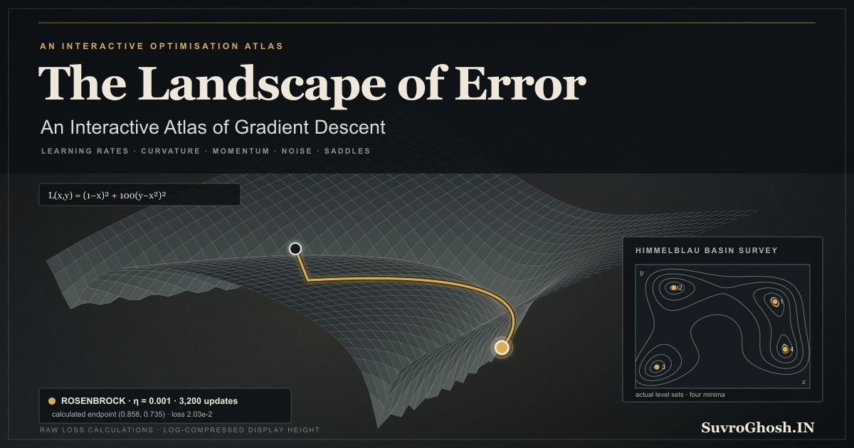
The Landscape of Error

An interactive atlas of gradient descent, learning rates, curvature, momentum, noise, saddles, and the peculiar geography of machine learning.

Drop a survey beacon anywhere. It has no map of the landscape; it can feel only the local slope beneath its feet.

Begin the descent Open the laboratory

Display height: log-compressed; calculations use raw loss.

LOW LOSSHIGH LOSS

Imagine being put down at midnight somewhere in the Himalayas without a map, a torch, or enough common sense to remain in the hotel. You are granted one useful sensation: through the soles of your boots you can feel the direction in which the ground falls most sharply. You may take a step, feel again, and repeat. You cannot see the valley beyond the next ridge. You do not know whether the lowest place in front of you is the lowest place in the range. You cannot even be sure that an almost level patch is a summit, a saddle, or merely a very tedious plateau.

This is roughly the predicament of gradient descent, except that gradient descent has no boots, no fear of leopards, and a frankly unhealthy willingness to repeat the same small calculation fifty million times.

The calculation is simple enough to fit in one line. Its consequences include cautious convergence, furious zig-zagging, overshooting, stagnation, escape, and the occasional arrival at a perfectly respectable minimum that happens not to be the best one available. The atlas below turns those consequences into geography without pretending that an optimiser is governed by gravity.

Gradient descent has no map of the landscape. It can feel only the local slope beneath its feet.

Audio article

Uses the speech voice supplied by your browser or device.

1. A walker with one sensation

A machine-learning model contains adjustable numbers called parameters. Collect them in a vector

For a straight line, the parameters might be its slope and intercept. For a neural network, they are weights and biases distributed through many layers. A loss function assigns one scalar number to a complete parameter setting:

Low loss means that the declared objective is being satisfied better. That sentence is deliberately narrower than “the model is better”. A training loss can omit costs we care about, reward a proxy that fails outside the sample, or improve while test performance deteriorates. The optimiser sees the mathematical objective it has been given, not the intentions of the person who wrote it.

The gradient is the vector of partial derivatives

At a differentiable point, the gradient points towards the direction of greatest local increase under the ordinary Euclidean notion of distance. Its negative points towards the steepest local decrease. “Local” is the expensive word. The gradient says what an infinitesimal move would do here; it does not provide a survey of what lies ten steps away.

In the atlas, two parameters are visible as the horizontal axes and loss is drawn vertically. The bright survey beacon is a parameter vector, not a ball. Its height is a display of $L(\boldsymbol{\theta})$, not physical altitude. It moves because an update equation changes the parameters, not because a graphics engine applies gravity.

Very tall peaks can flatten every useful valley in a literal-height drawing, so the terrain can use a labelled log-compressed display. It first shifts display loss by the robust sampled minimum and then plots a normalized $\log(1+max(0,L-L_{\min,\mathrm{sample}}))$. That shift makes negative-loss surfaces safe to draw. It never changes the raw loss, gradient, Hessian, stopping test, table, or export; changing the height switch changes the picture rather than the experiment.

Open the laboratory, choose the quadratic bowl, and drop the beacon somewhere away from the centre. The 3D terrain and the 2D contour map report the same function and the same point. Move the start on the contour map and both views must agree. If they do not, the exhibit is lying.

Interactive optimization observatory

The common instrument

Seven landscapes, four optimizers and one authoritative iteration clock. The contour map remains the complete scientific fallback if three-dimensional terrain is unavailable.

Load the interactive laboratory

2. One step, written carefully

Vanilla gradient descent uses

Here $t$ is an integer iteration count, $\mathbf{g}_t$ is the gradient evaluated at the current parameter vector, and $\eta>0$ is the learning rate. The actual update is

The distinction between gradient and update matters. The gradient belongs to the loss function at the current point. The update also depends on the optimiser, its internal state, and its hyperparameters. Momentum, RMSProp, and Adam can all receive the same gradient and produce different updates.

Press Single step and inspect the gradient and update arrows in the microscope. The gradient arrow points uphill because it represents $\mathbf{g}_t$; the update arrow points towards the next parameter setting. Their numerical components appear beside them, while the contour map shows the resulting path. That path joins a sequence of computed states. It is not a continuously solved trajectory, even when the marker is visually interpolated between two steps.

This makes the simulation clock pleasantly unromantic. An iteration is the scientific time step. Animation frames are merely opportunities to draw what has already been calculated. The learning rate is never multiplied by the time between frames. A slow phone and a fast desktop given the same landscape, start, settings, seed, and number of iterations must obtain the same path.

Reset is also a scientific operation. It restores the same start and the same seeded random streams. Replay follows the recorded experiment again. A new seed requests a different stochastic experiment; it must not be smuggled in merely because someone pressed Reset.

The path can end for several reasons, and “converged” is only one of them. The laboratory distinguishes convergence from an iteration limit, an escape from the displayed domain, numerical divergence, a stall near a stationary point, and an invalid parameter configuration. A stopped marker is an observation, not a certificate.

3. The learning rate is a wager

The learning rate converts a local derivative into a finite displacement. Too small, and the optimiser may make impeccable progress at the speed of municipal paperwork. Too large, and it can stride across the valley floor, climb the opposite wall, cross back with greater enthusiasm, or leave the finite numerical world altogether.

The rotated quadratic bowl makes this precise. Let

where $R$ is a rotation matrix and the eigenvalues $\lambda_1,\lambda_2$ are positive. Then

The Hessian $H$ is the matrix of second partial derivatives. For this exact positive-definite quadratic, its eigenvectors are the principal curvature directions and its eigenvalues say how sharply the loss bends along them. Vanilla gradient descent with a fixed learning rate is stable precisely within

A commonly optimal fixed step for this particular quadratic, judged by the worst contraction across its eigen-directions, is

These are not universal permission slips. A changing non-convex Hessian, noisy gradient, constraint, or different algorithm alters the analysis. The learning-rate gauge therefore presents the interval only for the quadratic chapter and labels it accordingly.

The ratio

is the condition number of this bowl. When $\kappa$ is close to one, its contours are nearly circular and a sensible step heads efficiently towards the centre. Increase $\kappa$ and the contours become long ellipses. A step chosen for the shallow direction becomes dangerous across the steep direction; a step safe across the walls barely advances along the floor. The resulting zig-zag is not indecision. It is the geometry of one scalar learning rate being asked to serve two very different curvatures.

The careful theory of descent methods extends far beyond this plate. Stephen Boyd and Lieven Vandenberghe make their book Convex Optimization freely available through Stanford; its unconstrained-minimisation chapters are a useful bridge from this two-dimensional bowl to line search, Newton steps, and convergence analysis.

4. Curvature makes a corridor

Select the Rosenbrock ravine:

with the classic values $a=1$ and $b=100$. Its gradient is

The minimum is at $(1,1)$, but the route there is a narrow curved valley. From the familiar starting point $(-1.2,1)$, an optimiser can descend quickly to the valley and then spend a long time crossing its walls while making modest progress along its bend. Being visually near the valley floor is not the same as being near the minimum in parameter space or loss.

H. H. Rosenbrock published “An Automatic Method for Finding the Greatest or Least Value of a Function” in 1960. The paper described a derivative-free minimisation method for a digital computer; the curved test problem that now bears his name became a durable way of embarrassing optimisation algorithms. Using it here does not imply that Rosenbrock invented gradient descent, nor that every machine-learning loss resembles a banana.

Turn on the local curvature ellipse and Hessian eigenvectors. One direction is sharply curved across the ravine; the other is much gentler along it. The gradient can point mostly towards the nearest part of the floor rather than along the long route to the optimum. Momentum may preserve useful motion along the valley, while an adaptive method may reduce updates in coordinates that have repeatedly received large gradients. Neither observation establishes a universal winner.

The one-dimensional cross-section in the microscope cuts through the current point along the actual optimiser update. It shows where that finite update sits relative to nearby loss along the direction the optimiser really chose; the separately drawn Hessian eigenvectors expose the principal-curvature directions. A tangent plane touches the surface at one point and records first-order information; it should not be mistaken for the terrain beyond that neighbourhood.

Display height deserves similar suspicion. Rosenbrock loss can vary so much across the visible domain that raw vertical scaling would turn its useful valley into a hairline beside a cliff. The atlas can log-compress height for legibility. The label states when it does so. Gradients, updates, loss readouts, stopping rules, and comparisons continue to use raw loss.

5. Four optimisers, one budget

An honest comparison begins with the same landscape, start, gradient-evaluation cap, stopping rule, and—where randomness is involved—the same declared data and seed. It does not give one optimiser a larger allowance because its line looks prettier after more work. A racer that meets the common stopping rule early may use fewer evaluations; the cards report actual evaluations as well as the shared cap, rather than padding the count with fictitious updates.

Vanilla gradient descent has no memory:

Momentum in this atlas uses one stated convention:

The accumulated vector $\mathbf{v}_{t+1}$ is algorithmic memory. It is not velocity generated by mass and gravity. Other books and libraries use related but differently scaled momentum conventions, so numerical hyperparameters should never be compared without first comparing definitions.

RMSProp maintains an element-wise moving average of squared gradients:

Squares, roots, and divisions here are element-wise. The denominator changes the effective scale of each coordinate. RMSProp was circulated in Geoffrey Hinton’s neural-networks course; the University of Toronto hosts the lecture notes describing the moving average of squared gradients. It is better described through that rule than through a retrofitted story in which the algorithm somehow perceives the whole landscape.

Adam combines moving averages of gradients and squared gradients. With $t$ beginning at one,

The powers in the bias corrections make an off-by-one error consequential at the beginning of a run. Kingma and Ba’s original Adam paper defines the moment estimates, their zero-initialisation bias, and the correction explicitly.

Run all four down Rosenbrock under the same budget, then change the learning rate. Momentum may travel smoothly at one setting and overshoot at another. Adam may make rapid early progress yet finish with a different path. RMSProp’s coordinate scaling can help with unequal gradient magnitudes, but it is not a device for discovering the global minimum. The atlas reports what happened in this experiment; it does not convert a four-line race into a general ranking of optimisers.

6. Many valleys and the politics of arrival

Himmelblau’s function has four well-known minima:

Release a grid of starts and the contour map becomes a flow field. Nearby points often converge to the same minimum, forming a basin of attraction for the selected optimiser and hyperparameters. The boundary is not a permanent property of the function alone. Change the learning rate, update rule, stopping tolerance, or noise model and some starts can cross into another basin, escape, or fail to settle within the budget.

The four reference minima are approximately

The basin map classifies a starting cell only when its run actually converges to a declared minimum. A cell that escapes the displayed domain, diverges numerically, or merely exhausts its budget receives its own non-colour pattern instead of being painted as a reluctant member of the nearest valley; the calculation summary reports how many have no declared destination. A cancellable worker keeps this survey away from the interface thread.

Rastrigin’s function is more corrugated:

Its global minimum is at the origin, but a regular array of local minima surrounds it. This landscape makes a blunt distinction visible: finding a minimum is not the same as finding the global minimum. A larger step or a noisy gradient may sometimes cross a ridge, but sometimes it crosses into a worse basin or diverges. Noise is not a moral force that delivers the marker to truth.

Particle flow is a census, not a swarm intelligence algorithm. Each beacon follows an independent copy of the stated optimiser from its own start. The pattern reveals attraction and sensitivity. It does not add interaction between particles, and the trajectories do not push or pull one another.

7. When almost still is not finished

Consider the contained saddle

Its gradient is

At the origin the gradient is exactly zero, but the point is not a minimum. The loss curves upwards along the $x$ direction and downwards along the $y$ direction. The Hessian has eigenvalues of opposite sign, making the local geometry saddle-like.

When numerical evidence is clear, Hessian eigenvalues provide a local classification. Two clearly positive eigenvalues are minimum-like; two clearly negative eigenvalues are maximum-like; opposite signs are saddle-like. Eigenvalues near zero make the result degenerate or inconclusive. A finite-difference Hessian, rounded coordinates, and floating-point arithmetic do not justify ceremonial confidence at the tolerance boundary.

Now move to the plateau

with

Far from the centre, the gradient can be extremely small even though a lower value remains elsewhere. The optimiser barely moves. A stopping rule based only on gradient norm may call this convergence; an iteration-limit status says something more modest. Loss change can also become tiny because the learning rate is tiny or floating-point resolution has swallowed the update.

This is why the laboratory exposes gradient norm, step norm, raw loss, iteration budget, and status together. None is a private channel to mathematical certainty. A stationary point is defined by first-order information. The kind of stationary point depends on local curvature, and the practical meaning of arrival depends on the model, precision, and objective.

8. A regression line becomes terrain

A loss landscape can sound metaphysical until an ordinary line produces one in front of us. Take data pairs $(x_i,y_i)$ and a model

There are two parameters, slope $m$ and intercept $b$, so the mean-squared-error objective is a genuine two-dimensional surface:

Its gradient is

Drag the regression line in the data view. The parameter beacon moves to the corresponding $(m,b)$ location on the contour map and terrain. Drag the beacon and the line must change in return. Residual segments show each vertical error; their squared lengths contribute to the bowl beneath the parameter point. Gradient descent turns a poor line into the least-squares fit by changing only $m$ and $b$.

Switch on the controlled outlier. One large residual enters the sum through its square, so its influence can dominate many smaller residuals. The bowl tilts and the least-squares optimum moves. The mathematics has not become malicious. Mean squared error was asked to penalise large residuals disproportionately, and it has complied. Robust losses answer a different modelling question; they are not silently substituted here.

The regression chapter also separates genuine minibatch gradients from illustrative noise. A batch of size $k$ computes the gradient of $k$ deterministically selected observations. It is an estimator of the full-data gradient, and its angular and magnitude errors can be measured against that reference. Batch sizes one, two, four, and full data therefore have an explicit data-generating meaning.

On a synthetic analytic landscape there is no hidden dataset from which to draw a minibatch. The optional experiment instead uses

where $\boldsymbol{\xi}_t$ is a seeded noise vector. The interface calls this a noisy-gradient experiment, not minibatch SGD. Identical seeds reproduce the sequence. Changing a decorative colour cannot advance it.

9. The step microscope

A path is easy to admire and surprisingly easy to misunderstand. The microscope pauses at one iteration and places the local quantities side by side:

• the current parameter vector $\boldsymbol{\theta}_t$;
• raw loss $L(\boldsymbol{\theta}_t)$;
• gradient $\mathbf{g}_t$ and its norm;
• the optimiser’s actual update $\Delta\boldsymbol{\theta}_t$ and its norm;
• optimiser memory, such as momentum or moment estimates;
• the Hessian and its eigenpairs when available;
• a tangent plane and one-dimensional loss profile;
• the learning-rate or hyperparameter state that produced the step.

The gradient and update need not be parallel. Momentum combines present and past gradients. RMSProp and Adam rescale coordinates. A minibatch estimate can point away from the full-data gradient. The microscope makes those differences visible rather than drawing one ambiguous arrow labelled “direction”.

The Hessian is local as well. For a twice-differentiable loss, a second-order approximation around $\boldsymbol{\theta}$ is

The linear term supplies the tangent plane; the quadratic term supplies local bending. This approximation can be excellent for a small displacement and dreadful beyond a nearby turn in the valley. Showing it beside the true one-dimensional profile is a useful antidote to treating Taylor expansion as aerial photography.

Accessibility requires another representation of the same evidence. Colour is never the only identity channel: optimiser paths also differ by line pattern and marker shape. Controls have visible labels and keyboard operation. The current values and run status exist as text. The principal path samples can be read in a table and exported as CSV; a short plain-text summary copies the disclosed configuration and outcome. Reduced-motion mode begins still, while manual stepping, changing views, and inspecting the table remain available.

10. What the pretty map hides

Every landscape on this page is exact within its declared two-dimensional model and numerical implementation. That does not make it a literal portrait of a modern neural network.

A network with $d$ parameters has a loss defined over $\mathbb{R}^d$. When $d$ is in the millions, a two-dimensional picture can show only two chosen directions, a projection, or a deliberately small surrogate. Directions invisible to the plane may contain sharp curvature, flat symmetries, barriers, or escape routes. Reparameterising a model can change the apparent geometry even when its computed function remains equivalent. Axes with unlike scales can make visual steepness depend on units.

Hao Li, Zheng Xu, Gavin Taylor, Christoph Studer, and Tom Goldstein discuss these problems in Visualizing the Loss Landscape of Neural Nets. Their filter-normalisation method was introduced because naive random-direction plots can make comparisons misleading. A loss-landscape image is an experiment with choices, not a window opened directly onto an otherwise invisible object.

The atlas also displays training loss, not generalisation. Two parameter settings with similar training loss may behave differently on unseen data. A flatter-looking minimum in one chosen slice is not by itself proof of better generalisation. Adam reaching a low point quickly in this laboratory is not a guarantee that Adam is preferable for a different architecture, dataset, budget, regularisation scheme, or metric.

There is, nevertheless, something historically durable in the small local step. In 1847 Augustin-Louis Cauchy published Méthode générale pour la résolution des systèmes d’équations simultanées in volume 25 of the Comptes rendus de l’Académie des sciences, pages 536–538. Modern histories trace the method of steepest descent to that note, in which a sum-of-squares problem for simultaneous equations is reduced by following a direction of steepest local decrease. Cambridge’s edition of Cauchy’s collected works provides the reprinted note and bibliographic record. The fixed-learning-rate machine-learning update used today is a descendant of that construction, not a verbatim transcription of a nineteenth-century algorithm.

Cauchy’s optimiser had no GPU terrain, no Adam comparison, and no button marked Release many starts. It faced the same fundamental economy of information. At a point, calculate what the function says locally. Choose how far to trust that message. Move. Measure again.

The surface may be a bowl, ravine, saddle, plateau, or slice through something too large to picture. The optimiser still has no map.

It has a slope, a memory if we give it one, a budget, and the next step.

Sources and further reading. Augustin-Louis Cauchy, Méthode générale pour la résolution des systèmes d’équations simultanées (1847); H. H. Rosenbrock, An Automatic Method for Finding the Greatest or Least Value of a Function (1960); Stephen Boyd and Lieven Vandenberghe, Convex Optimization (2004); Tijmen Tieleman and Geoffrey Hinton, RMSProp lecture notes; Diederik P. Kingma and Jimmy Ba, Adam: A Method for Stochastic Optimization; Hao Li and colleagues, Visualizing the Loss Landscape of Neural Nets.