Linear Algebra: The Hidden Architecture of Machine Learning

Audio article

Uses the speech voice supplied by your browser or device.

A glowing geometric grid of interconnected nodes and vector planes in indigo and violet

Linear Algebra: The Hidden Architecture of Machine Learning

The Quiet Tyrant

I did not choose to care about linear algebra.

Nobody does, at first.

You sit in a fluorescent-lit classroom, perhaps sophomore year, perhaps bleary-eyed at 9 AM, and a professor writes something on a whiteboard that looks like a crossword puzzle designed by a sadist: a grid of numbers, bracketed, labeled with subscripts that seem to multiply like bacteria. You are told to “find the eigenvalues.” You are told that this matters. You nod, you copy, you calculate determinants by hand until your fingers cramp, and you wonder—honestly, genuinely wonder—whether this is some elaborate hazing ritual perpetrated by the mathematics department upon the innocent.

I thought this.

I thought this for years.

And then, one afternoon, I watched a neural network learn to recognize a cat.

Not a metaphorical cat. An actual cat. A tabby, specifically, curled on a windowsill, bathed in afternoon light, its fur a texture map of orange and black stripes. The network had never seen this particular cat before. It had seen millions of other cats—Siamese, Persian, hairless Sphynxes with their unsettling, wrinkled elegance—but not this one. Yet it knew. It output, with 94.7% confidence, the word “cat.”

And I realized, with the slow, dawning horror of someone who has just discovered that the foundation of their house is made of something alive and breathing, that every single operation that made this recognition possible—every weight, every bias, every forward pass and backward propagation—was, at its core, an act of linear algebra.

Not calculus, though calculus was there, lurking in the background like a stage manager.

Not probability, though probability provided the costume.

Linear algebra.

The quiet tyrant.

The hidden architecture.

The invisible scaffolding upon which the entire cathedral of modern machine learning has been constructed, beam by beam, vector by vector, matrix multiplication by matrix multiplication, until what began as an abstract game with numbers in grids has become the engine that translates languages in milliseconds, generates images from whispers of text, recommends your next song with eerie precision, and drives cars through streets it has never physically traversed.

This is the story of that scaffolding.

This is the story of why you should care, even if you think you shouldn’t, even if you think mathematics is a language spoken only by the initiated in ivory towers, even if you believe—erroneously, but understandably—that linear algebra is merely a prerequisite to be survived rather than a worldview to be embraced.

I am going to take you from the very beginning.

From the ancient Babylonians scratching clay tablets.

To the vector spaces that breathe inside your phone.

We will move in concentric circles, spiraling inward, from the broad historical sweep to the electron-level specifics, and I promise you—genuinely promise—that by the end, you will not merely understand linear algebra; you will feel it, the way a musician feels rhythm or a sailor feels the tide.

Let us begin.

Who Is Involved? The Dramatis Personae of Abstraction

The cast of characters in this story is improbably vast, stretching across millennia and continents, from scribes in Mesopotamia to programmers in Palo Alto, from philosophers contemplating the nature of space to engineers optimizing the throughput of GPU clusters.

Let me introduce them.

The Ancient Practitioners. Around 2000 BCE, Babylonian scribes were already solving systems of what we would now recognize as linear equations—problems involving multiple unknown quantities related by linear constraints—though they expressed them in the concrete language of geometry and commerce: fields to be divided, grain to be distributed, inheritances to be allocated. They did not know they were doing linear algebra. They were simply solving problems. The abstraction would come later, like a shadow slowly lengthening as the sun descends.

The Chinese Mathematicians. By the 2nd century BCE, Chinese mathematicians had developed sophisticated methods for solving systems of linear equations, documented in texts like the Jiuzhang Suanshu (Nine Chapters on the Mathematical Art). Their “fangcheng” method—literally “rectangular arrangement”—involved arranging coefficients in a grid and manipulating rows to eliminate variables. They were performing Gaussian elimination two millennia before Gauss was born, which is either a testament to the universality of mathematical insight or a rather embarrassing oversight in Western historiography, depending on your perspective.

The Persian Polymaths. In the 9th century CE, Muhammad ibn Musa al-Khwarizmi—whose name, Latinized, gives us the word “algorithm”—systematized the solution of linear equations in his treatise Al-Kitab al-Mukhtasar fi Hisab al-Jabr wal-Muqabala (The Compendious Book on Calculation by Completion and Balancing). The word “algebra” itself derives from “al-jabr,” meaning “reunion of broken parts.” Al-Khwarizmi was not thinking about neural networks. He was thinking about inheritance law and land measurement. But he was laying the grammatical foundations of a language that would, twelve centuries later, describe the structure of artificial intelligence.

The Renaissance Geometers. Descartes, in the 17th century, gave us the coordinate system—the Cartesian plane—that allowed geometry to be expressed algebraically. This was revolutionary. Before Descartes, a line was a geometric object, drawn with compass and straightedge. After Descartes, a line was an equation: y = mx + b. The marriage of geometry and algebra was consummated, and their child—analytic geometry—would grow up to be the parent of linear algebra.

The 19th-Century Revolutionaries. Here is where the story accelerates, where characters appear in rapid succession, each adding a crucial piece to the puzzle. Grassmann (Hermann Grassmann, 1809–1877), a German schoolteacher and Sanskrit scholar, developed the theory of vector spaces in his Ausdehnungslehre (Theory of Extension) in 1844. His work was so abstract, so ahead of its time, that it was largely ignored during his lifetime. He introduced the concept of an n-dimensional space—a space with not just the three dimensions we can see, but four, five, a hundred, a million dimensions. The reviewers of his time found his work “obscure.” They were not wrong; it was obscure. But it was also correct, and essential.

Cayley and Sylvester (Arthur Cayley and James Joseph Sylvester, mid-19th century) gave us the word “matrix”—from the Latin for “womb” or “source”—and developed matrix algebra, including the determinant and the inverse. Cauchy (Augustin-Louis Cauchy) systematized much of the terminology. Hamilton (William Rowan Hamilton) discovered quaternions, a four-dimensional number system that would prove crucial for 3D computer graphics and, by extension, the spatial reasoning of modern AI.

The 20th-Century Formalizers. By the early 1900s, linear algebra had matured from a collection of techniques into a rigorous, axiomatic theory. David Hilbert and Stefan Banach developed the theory of Hilbert spaces and Banach spaces—infinite-dimensional vector spaces with additional structure (inner products and norms, respectively) that became essential for quantum mechanics and, later, for the mathematical foundations of machine learning. Emmy Noether, perhaps the most important mathematician you have never heard of, revolutionized abstract algebra and showed how algebraic structures underlie physical conservation laws. Her work on modules and rings provided the categorical framework that allows modern linear algebra to generalize across seemingly disparate domains.

The Computer Scientists and Engineers. In the mid-20th century, as digital computers emerged from the theoretical ether into physical reality, linear algebra found its ultimate practical expression. John von Neumann, the polymath’s polymath, understood that computers were essentially machines for performing matrix operations at scale. Gene Golub developed numerical methods for matrix computation—algorithms that could solve linear systems efficiently and stably on finite-precision machines. Jack Dongarra created the LAPACK and BLAS libraries, the foundational software upon which virtually all modern scientific computing rests.

The Machine Learning Pioneers. Frank Rosenblatt invented the Perceptron in 1957—a single-layer neural network that learned weights through linear classification. Geoffrey Hinton, Yann LeCun, and Yoshua Bengio—the “Godfathers of Deep Learning”—spent decades developing the multi-layer architectures that depend, at every layer, on matrix multiplications. Fei-Fei Li built ImageNet, the dataset that proved deep learning could work at scale, and every image in that dataset was represented as a matrix of pixel values, every convolutional filter as a small matrix sliding across that image, every feature map as the result of matrix operations.

And then there is you.

Yes, you.

The person reading this, perhaps on a device whose screen is illuminated by billions of matrix operations per second, perhaps wondering whether this journey into abstraction will be worth the effort. You are part of this story now. You are about to become one of the initiated, one of the people who can look at a neural network and see not a black box, not magic, but a beautifully structured sequence of linear transformations, nonlinear activations, and gradient descents through high-dimensional vector spaces.

The cast is assembled.

The stage is set.

Let us understand what, exactly, they have built.

What Is It? The Essence of Linear Algebra

Linear algebra is the mathematics of linearity.

This sounds tautological, and in a sense it is, but let me unpack it, because the concept of linearity is both more specific and more profound than it first appears.

At its most fundamental level, linear algebra studies mathematical objects called vectors and the rules by which they can be combined and transformed, and it does so in a way that preserves a very particular kind of structure: the structure of straight lines, flat planes, and their higher-dimensional analogues.

A vector, in the most concrete sense, is an ordered list of numbers. You can think of it as an arrow in space—pointing from the origin to some coordinate—or as a point in space itself, or as a packet of data, or as a direction with magnitude. The beauty of linear algebra is that all these interpretations are simultaneously valid and mutually illuminating.

In machine learning, a vector might represent:

The pixel values of an image (a 784-dimensional vector for a 28×28 grayscale image)
The word embeddings of a vocabulary term (a 300-dimensional vector in Word2Vec)
The features of a customer (age, income, purchase history, all stacked into a vector)
The hidden state of a neural network layer (a 2048-dimensional vector in a large language model)

A matrix is a rectangular grid of numbers—an arrangement of vectors, either as rows or columns. It is the most fundamental data structure in linear algebra, and in machine learning, matrices are everywhere: datasets are matrices (rows are samples, columns are features), weights in neural networks are matrices, images are matrices of pixel values, adjacency graphs are represented as matrices, and the entire training process of deep learning is, at its core, a sequence of matrix multiplications.

But linear algebra is not merely about vectors and matrices as static objects. It is about transformations—about what happens when you multiply a vector by a matrix, when you multiply matrices together, when you decompose matrices into simpler components.

And here is where the concept of linearity becomes crucial.

A transformation is linear if it satisfies two properties:

Additivity: T(u + v) = T(u) + T(v) — transforming the sum of two vectors equals the sum of their individual transformations.
Homogeneity: T(c·v) = c·T(v) — scaling a vector before transformation equals scaling it after.

In plain language: linear transformations preserve the operations of vector addition and scalar multiplication. They keep straight lines straight. They keep the origin fixed. They do not bend, twist, or warp space in nonlinear ways. They stretch, rotate, reflect, project, and shear—but they do so uniformly, predictably, structurally.

This might sound restrictive. It is. But here is the profound insight that makes linear algebra the language of machine learning: locally, almost everything is linear.

Calculus tells us that any sufficiently smooth function can be approximated by a linear function in a small enough neighborhood. A neural network with its nonlinear activation functions is globally nonlinear—capable of learning the twisted, warped, bizarrely shaped decision boundaries that separate cats from dogs, spam from ham, malignant tumors from benign growths. But during training, during the forward pass and the backward pass, we are constantly computing linear approximations. The gradient—the direction of steepest descent—is a linear concept. The Jacobian matrix of partial derivatives is a linear operator. Even the most complex deep network is, at the level of a single layer, a linear transformation followed by a nonlinear “squashing” function.

Linear algebra, then, is the grammar of machine learning. It is the syntax that allows us to express complex ideas—“rotate this high-dimensional space so that the classes are separable,” “project this text into a semantic space where similar meanings cluster,” “find the principal directions of variation in this dataset”—in a language that computers can execute at billions of operations per second.

But to truly understand what linear algebra is, we must understand where it came from, when it emerged from the concrete into the abstract, from the specific to the general, from the Babylonian field division to the infinite-dimensional Hilbert spaces that describe quantum states and, increasingly, the latent spaces of generative AI.

When Did It Emerge, Evolve, and Become Significant? A Timeline of Abstraction

The history of linear algebra is not a straight line. It is a braided river, with tributaries flowing from geometry, from algebra, from physics, from engineering, converging and diverging, sometimes drying up for centuries only to flood forth with renewed vigor when the intellectual climate changed.

Let me trace this river.

The Ancient Confluence (2000 BCE – 300 CE)

The earliest linear algebra was invisible. It was not called linear algebra. It was called “solving practical problems.” Babylonian clay tablets from around 2000 BCE contain problems like: “There are two fields whose total area is 1800 square units. One produces grain at 2/3 of a unit per square unit, the other at 1/2. The total yield is 1100 units. Find the areas of the fields.” This is a system of two linear equations in two unknowns. The scribes solved them using methods equivalent to what we now call substitution and elimination.

The Chinese, as mentioned, systematized this in the Nine Chapters, developing a method of arranging coefficients in columns and performing row operations—what we now call Gaussian elimination, though Gauss would not be born for another two millennia. The Chinese even recognized that some systems had no solution (inconsistent) or infinitely many solutions (dependent), concepts that would not be fully formalized in the West until the 19th century.

These were the headwaters: concrete, practical, tied to the earth and its measurement.

The Islamic Golden Age (800–1400 CE)

Al-Khwarizmi’s Al-Jabr (c. 820 CE) gave the world the word “algebra” and a systematic approach to solving linear equations. His methods were rhetorical—he wrote out procedures in words, not symbols—but they were general. He classified linear equations into six types and gave algorithmic solutions for each. The word “algorithm” itself derives from his name, a fitting etymology given that modern machine learning is, at its core, a sequence of algorithmic linear algebraic operations.

During this period, the connection between algebra and geometry remained implicit. Algebra was a tool for solving equations; geometry was a separate realm of shapes and proofs. They had not yet merged into the unified discipline that would become analytic geometry and, eventually, linear algebra.

The Cartesian Revolution (1637)

René Descartes published La Géométrie in 1637 as an appendix to his Discourse on the Method, and the world changed—not immediately, not for everyone, but fundamentally and irrevocably. Descartes showed that geometric problems could be translated into algebraic equations and solved algebraically, then translated back into geometric results.

A line was no longer just a line. It was an equation. A curve was no longer just a curve. It was a function. The two-dimensional plane became a coordinate system, a grid of numbers where every point had an address (x, y), and every geometric object had an algebraic representation.

This was the birth of what we now call the vector space—though the term would not be coined for another two centuries. The plane became R², the set of all ordered pairs of real numbers. Space became R³, the set of all ordered triples. And though Descartes himself did not venture into higher dimensions, he had opened the door. Once you realize that space can be described by numbers, it is a short conceptual leap—though historically, it took two hundred years—to ask: why stop at three?

The 19th Century: The Birth of Modern Linear Algebra (1840–1900)

This is where the river floods.

1844: Grassmann’s Ausdehnungslehre. Hermann Grassmann, a German schoolteacher with a side interest in Sanskrit linguistics, published a work so abstract, so general, so far ahead of its time that it was essentially ignored. He defined vector spaces of arbitrary dimension. He introduced the exterior product and the inner product. He developed a theory of linear transformations that applied not just to geometry but to any domain where objects could be added and scaled.

Grassmann’s work was a masterpiece of clarity and obscurity—clear in its logic, obscure in its reception. He was not a professional mathematician. He was a schoolteacher. The mathematical establishment found his ideas bizarre, unnecessary, overly abstract. It would take decades for the world to catch up.

1858: Cayley’s Memoir on the Theory of Matrices. Arthur Cayley, a British mathematician, published the first systematic treatment of matrices as algebraic objects in their own right, not merely as convenient arrangements of coefficients. He defined matrix multiplication, the inverse matrix, and the determinant. He showed that matrices could represent linear transformations and that the composition of transformations corresponded to matrix multiplication.

This was crucial. Before Cayley, a matrix was just a grid of numbers—a bookkeeping device. After Cayley, a matrix was an operator, an actor upon the stage of vector space, capable of rotating, stretching, projecting, and reflecting entire spaces with a single multiplication.

1870s–1880s: The Development of Determinants and Eigenvalues. The concepts of the determinant (a scalar value that encodes whether a matrix is invertible, whether a transformation collapses space) and the eigenvalue (a special scaling factor associated with particular directions that remain unchanged under transformation) were refined and generalized. The German word Eigenwert—“own value”—was coined, and the English “eigenvalue” followed, giving us one of the most important concepts in all of applied mathematics.

Eigenvalues and eigenvectors would prove essential not just for physics (where they describe the natural frequencies of vibrating systems, the energy levels of quantum states) but for machine learning, where they underlie Principal Component Analysis (PCA), spectral clustering, PageRank, and the stability analysis of neural networks.

1888: Peano’s Axioms. Giuseppe Peano, the Italian mathematician famous for his space-filling curve, provided the first modern axiomatic definition of a vector space. He listed the properties that a collection of objects must satisfy to be considered a vector space: closure under addition and scalar multiplication, associativity, commutativity, the existence of zero and inverse elements, and the distributive properties.

This was the moment when linear algebra became truly abstract. No longer tied to arrows in space or grids of numbers, a vector space could be any collection of objects—functions, polynomials, quantum states, images, words—provided they satisfied Peano’s axioms. The theory became universal, applicable across domains, a true mathematical language rather than a specific technique.

The 20th Century: From Physics to Computers to AI (1900–2000)

Quantum Mechanics and Hilbert Spaces (1920s–1930s). The development of quantum mechanics required a mathematical framework for describing physical systems with infinitely many degrees of freedom. David Hilbert and John von Neumann developed the theory of Hilbert spaces—infinite-dimensional vector spaces equipped with an inner product that allows the definition of angles and distances.

In quantum mechanics, the state of a system is a vector in a Hilbert space. Observables (position, momentum, energy) are linear operators (matrices, in the finite-dimensional case) acting on that space. The eigenvalues of these operators are the possible measurement outcomes. The entire edifice of quantum theory is built upon linear algebra.

This would have profound implications for machine learning, though those implications would not become fully apparent for nearly a century. The concept of a state vector—a complete description of a system encoded as a vector in a high-dimensional space—would reappear in the hidden states of recurrent neural networks, in the embeddings of natural language processing, in the latent vectors of generative models.

The Digital Revolution and Numerical Linear Algebra (1940s–1970s). The invention of digital computers transformed linear algebra from a theoretical discipline into a practical engineering tool. During World War II and the Cold War, computers were used to solve large systems of linear equations arising from physics simulations, structural engineering, and cryptography.

Gene Golub and others developed algorithms for matrix computation that were both efficient (running in reasonable time) and stable (not exploding with rounding errors). The QR decomposition, the singular value decomposition (SVD), and iterative methods for solving large sparse systems were developed and refined. The BLAS (Basic Linear Algebra Subprograms) and LAPACK libraries standardized these algorithms, making them available across platforms.

The Rise of Machine Learning (1950s–2000s). Frank Rosenblatt’s Perceptron (1957) was a linear classifier—a single matrix multiplication followed by a threshold function. The backpropagation algorithm, developed in the 1970s and popularized in the 1980s, used the chain rule of calculus to compute gradients through networks, and those gradients were vectors, the weight updates were matrix operations, and the entire training process was a sequence of linear algebraic computations.

The “AI winter” of the late 1980s and 1990s saw reduced interest in neural networks, but linear algebra continued to power other machine learning methods: support vector machines (which find optimal separating hyperplanes in high-dimensional spaces), principal component analysis (which uses eigenvalue decomposition to reduce dimensionality), latent semantic analysis (which uses SVD to discover hidden topics in text), and collaborative filtering (which uses matrix factorization to recommend movies and products).

The Deep Learning Explosion (2006–Present)

In 2006, Geoffrey Hinton and his colleagues published papers showing that deep belief networks could be trained effectively using a technique called layer-wise pretraining. The deep learning revolution had begun, and it was powered by linear algebra at every level.

GPUs (Graphics Processing Units), originally designed for rendering 3D graphics using matrix operations, proved to be ideally suited for the matrix multiplications that dominate deep learning. Companies like NVIDIA pivoted from gaming to AI, and the CUDA programming language allowed researchers to perform massive parallel matrix operations on thousands of cores simultaneously.

AlexNet (2012), the convolutional neural network that won the ImageNet competition by a massive margin, used millions of matrix multiplications in its convolutional and fully connected layers. Word2Vec (2013) represented words as vectors in a high-dimensional space where semantic relationships became geometric relationships: king - man + woman ≈ queen. Transformers (2017), the architecture behind GPT and BERT, are essentially elaborate mechanisms for computing attention—a weighted combination of vectors, where the weights are themselves computed by matrix multiplications.

GPT-4, Claude, Gemini—the large language models that have captured the public imagination—are, at their core, sequences of matrix multiplications interspersed with nonlinear activation functions. When you type a prompt into ChatGPT, your text is converted into vectors (embeddings), those vectors are multiplied by weight matrices, transformed, multiplied again, passed through attention mechanisms that are themselves matrix operations, and finally projected back into the space of possible next tokens.

Billions of parameters. Billions of matrix entries. Billions of floating-point operations per second.

All linear algebra.

All the time.

Where Does It Occur, Operate, and Apply? The Geography of Vector Space

Linear algebra operates everywhere, which is both a banal statement and a profound one. Let me be more specific, more geographical, more attuned to the particular landscapes where linear algebraic thinking dominates.

The Landscape of Data Science

In data science, every dataset is a matrix. Rows are observations. Columns are features. A dataset of 10,000 customers with 50 attributes each (age, income, purchase history, website clicks, etc.) is a 10,000 × 50 matrix. The fundamental operations of data science—standardization (subtracting the mean and dividing by the standard deviation), principal component analysis (finding the directions of maximum variance), linear regression (finding the hyperplane that best fits the data)—are all linear algebraic operations.

When a data scientist says “let’s reduce the dimensionality of this dataset,” they are proposing to find a lower-dimensional subspace—a smaller vector space embedded within the larger one—that captures most of the important variation. This is linear algebra. When they say “let’s cluster these points,” they are often proposing to measure distances in vector space and group nearby points together. Distance in vector space is defined by the norm—a linear algebraic concept.

The Terrain of Computer Graphics and Vision

Every image on your screen is a matrix. A grayscale image is a 2D matrix of pixel intensities. A color image is a 3D tensor (a generalization of a matrix to higher dimensions) with three channels: red, green, blue. When Photoshop applies a filter, it is performing convolution—sliding a small matrix (the kernel) across the image matrix and computing dot products at each position. When Instagram applies a “vintage” filter, it is multiplying pixel values by matrices that adjust color balance, contrast, and saturation.

In computer vision, convolutional neural networks (CNNs) use learned convolutional filters—small matrices that detect edges, textures, shapes, and increasingly abstract features as you move deeper into the network. The famous AlexNet architecture uses five convolutional layers, each performing thousands of convolutions (matrix operations) per image. The feature maps at each layer are matrices. The weights are matrices. The activations are vectors.

When a self-driving car “sees” a pedestrian, it is not seeing in any human sense. It is performing a cascade of matrix multiplications on pixel values, transforming the raw image into increasingly abstract representations, until a final layer outputs a vector of probabilities: [0.02, 0.01, 0.87, 0.10]—car, tree, pedestrian, bicycle.

The Domain of Natural Language Processing

Language, that most human of faculties, has been colonized by linear algebra.

In early NLP, words were represented as one-hot vectors: a vector with a 1 in one position and 0 everywhere else, with the position corresponding to the word’s index in a vocabulary. “Cat” might be [0, 0, 0, 1, 0, 0, …] and “dog” [0, 0, 0, 0, 1, 0, …]. These vectors are high-dimensional (vocabulary size, often 10,000–100,000) and utterly uninformative about meaning. The dot product of “cat” and “dog” is zero. They are orthogonal, perpendicular, unrelated in vector space.

Word embeddings changed everything. In 2013, Tomas Mikolov and his colleagues at Google developed Word2Vec, a neural network that learns to represent words as dense vectors in a lower-dimensional space (typically 100–300 dimensions) such that words with similar meanings are close together. “Cat” and “dog” are no longer orthogonal. They are nearby vectors, separated by a small angle, because they appear in similar contexts.

The famous analogy: king - man + woman ≈ queen.

This is not magic. It is geometry. In the vector space of Word2Vec, the vector from “man” to “king” (king - man) captures the concept of “royalty.” Adding this vector to “woman” yields a vector near “queen.” The relationships between words have become linear relationships between vectors.

Modern large language models use contextual embeddings—vectors that depend not just on the word itself but on its surrounding context. BERT, GPT, T5—all of them convert text into vectors, process those vectors through layers of matrix multiplications and attention mechanisms, and output new vectors that represent probabilities over the next token, or answers to questions, or classifications of sentiment.

The attention mechanism, introduced in the 2017 paper “Attention Is All You Need,” computes a weighted sum of value vectors, where the weights are determined by the similarity (dot product) between query and key vectors. It is, fundamentally, a mechanism for routing information through vector space, for allowing different parts of a sequence to “talk” to each other by measuring their alignment in high-dimensional space.

The Atmosphere of Physics and Engineering

Linear algebra is the native language of physics. Quantum mechanics represents states as vectors in Hilbert space and observables as operators (matrices). The Schrödinger equation is a linear partial differential equation. General relativity uses tensors—generalizations of matrices that transform in specific ways under coordinate changes.

In control theory, the behavior of dynamic systems (airplanes, robots, chemical plants) is modeled using systems of linear differential equations, solved using matrix exponentials and eigenvalue analysis. In signal processing, the Fourier transform decomposes signals into sinusoidal components, and the discrete Fourier transform is computed efficiently using the Fast Fourier Transform (FFT) algorithm, which is essentially a factorization of a matrix into sparse matrices.

In structural engineering, the finite element method discretizes continuous structures into meshes, and the equilibrium equations become large sparse linear systems solved using iterative matrix methods. In electrical engineering, circuit analysis uses Kirchhoff’s laws to set up systems of linear equations, solved via matrix inversion.

The Stratosphere of Pure Mathematics

Even in the rarefied air of pure mathematics, linear algebra is omnipresent. Algebraic topology uses linear algebra to count holes in shapes (homology groups are vector spaces). Differential geometry studies curved spaces by approximating them locally with flat (linear) spaces (tangent spaces). Representation theory studies abstract algebraic structures by representing their elements as matrices. Functional analysis extends linear algebra to infinite-dimensional spaces, providing the rigorous foundation for quantum mechanics and partial differential equations.

Why Does It Matter? The Stakes of the Invisible

Why should you care about linear algebra?

I can give you the practical answer, and I will, but first let me give you the philosophical one, because the practical answer, while true, is insufficient.

The Philosophical Answer: The Geometry of Thought

Linear algebra matters because it provides a framework for understanding structure.

When we look at the world, we see objects, relationships, patterns, causes, and effects. But beneath these appearances, there is structure—mathematical structure—that persists across domains. Linear algebra is the study of one of the most fundamental kinds of structure: the structure of spaces where things can be added and scaled, where straight lines remain straight, where the whole can be understood as the sum of its parts in a precise, formal sense.

The vector space is one of the most important abstract structures in all of mathematics because it captures the essence of combination and proportion. Any system where you can combine things and scale them—where 2x + 3y makes sense—is a vector space. This includes:

Physical forces (vector addition of forces)
Colors (mixing red and blue to get purple)
Sounds (superposition of sound waves)
Financial portfolios (combinations of assets)
Chemical mixtures (proportions of reactants)
Genetic expressions (combinations of gene activities)
Word meanings (combinations of semantic features)
Neural activations (combinations of neuron firings)

Linear algebra teaches us that all these domains, despite their surface differences, share a deep structural similarity. They are all vector spaces. They all obey the same rules. They can all be analyzed with the same tools.

This is not just useful. It is profound. It is a manifestation of what the physicist Eugene Wigner called “the unreasonable effectiveness of mathematics in the natural sciences”—the mysterious fact that abstract mathematical structures, invented by human minds for reasons of logical beauty and internal consistency, turn out to describe the physical world with astonishing accuracy.

Linear algebra is unreasonable in this way. Grassmann invented vector spaces in 1844 as an abstract theory of extension. A century and a half later, those same vector spaces describe the semantic relationships between words in natural language, the feature hierarchies in deep neural networks, and the quantum states of elementary particles. The same structure. The same mathematics. Applied to domains that Grassmann could not have imagined.

This suggests something deep about the nature of reality and the nature of mind. It suggests that linearity—additivity and homogeneity, the preservation of structure under combination and scaling—is not just a mathematical convenience but a fundamental feature of how the universe organizes itself, from the quantum level to the cognitive level.

The Practical Answer: The Engine of Modern AI

But let me descend from the philosophical stratosphere to the practical terrain, because the practical stakes are also enormous.

If you want to understand machine learning—not just use it as a black box, not just call model.fit() and hope for the best, but actually understand why it works, why it fails, how to improve it, how to debug it, how to innovate upon it—you need linear algebra.

Here is why:

Understanding architectures. When you read a paper proposing a new neural network architecture—“We introduce the XYZ-Net, which uses a novel attention mechanism based on orthogonal projections in a learned subspace”—every term in that sentence is a linear algebraic concept. Orthogonal projections. Learned subspaces. If you do not know what these mean, you cannot understand the paper, cannot implement the model, cannot extend the idea.

Debugging and optimization. When your model is not training—when the loss is NaN, when the gradients are exploding, when the activations are vanishing to zero—you need to understand the linear algebraic properties of your network. Is the weight matrix singular? Are the eigenvalues of the Hessian causing optimization instability? Is the condition number of your data matrix causing numerical issues? These are not esoteric concerns. They are the daily bread of the machine learning engineer.

Efficient implementation. When you deploy a model to production, every matrix multiplication matters. Understanding the computational complexity of matrix operations—knowing that multiplying two n × n matrices takes O(n³) time with standard algorithms, or O(n²·³⁷³) with the fastest known theoretical algorithms, or that sparse matrix operations can be much faster—allows you to optimize your code, choose appropriate batch sizes, design efficient architectures, and avoid bottlenecks.

Innovation. The most important advances in machine learning often come from new linear algebraic insights. The Transformer architecture (2017) was revolutionary because it replaced recurrent connections (sequential, slow) with attention mechanisms (parallelizable, matrix-based). Graph neural networks use linear algebra on adjacency matrices to propagate information through networks. Normalizing flows use invertible linear transformations to map between simple and complex distributions. Diffusion models use linear algebra to gradually denoise images in a high-dimensional vector space.

If you do not understand linear algebra, you are not a machine learning practitioner. You are a machine learning user. There is nothing wrong with being a user—most people are users of most technologies—but if you aspire to build, to innovate, to push the boundaries, you need the language.

The Economic Answer: The Currency of the AI Economy

The global AI market is projected to reach trillions of dollars in the coming decades. Every major technology company—Google, Microsoft, Amazon, Meta, NVIDIA, OpenAI, Anthropic, DeepMind—employs thousands of people whose daily work consists of manipulating matrices, optimizing matrix multiplications, and designing new linear algebraic architectures.

NVIDIA, the most valuable company in the world by market capitalization (at times), sells GPUs—machines designed specifically for performing matrix operations in parallel. Their entire business model is built on the fact that modern AI is linear algebra at scale.

Understanding linear algebra is not just intellectually enriching. It is economically valuable. It is the difference between being a consumer of AI and being a producer of AI. Between being affected by the technological revolution and being an agent within it.

How Does It Work? The Mechanisms, From Surface to Depth

Now we descend into the mechanisms. This is where the abstract becomes concrete, where definitions become operations, where the “what” and “why” give way to the “how.”

I will proceed in concentric circles, from the most basic operations to the most sophisticated, from the surface to the depths, from the bird’s eye view to the electron level.

Circle One: Vectors and the Basic Operations

A vector is an ordered list of numbers. In machine learning, we typically work with column vectors—vectors arranged vertically:

$\mathbf{v} = \begin{bmatrix} v_1 \\ v_2 \\ \vdots \\ v_n \end{bmatrix}$

Vectors live in vector spaces. The most common vector space in machine learning is Rⁿ—the space of all n-dimensional vectors with real number entries. If n = 2, this is the plane. If n = 3, this is ordinary space. If n = 768, this is the hidden dimension of BERT-base, a space no human can visualize but which contains rich semantic structure.

Vector addition is performed component-wise:

$\mathbf{u} + \mathbf{v} = \begin{bmatrix} u_1 + v_1 \\ u_2 + v_2 \\ \vdots \\ u_n + v_n \end{bmatrix}$

Geometrically, this is the parallelogram law: place the tail of v at the head of u, and the sum is the diagonal from the origin to the far corner.

Scalar multiplication multiplies every component by a number:

$c \mathbf{v} = \begin{bmatrix} c v_1 \\ c v_2 \\ \vdots \\ c v_n \end{bmatrix}$

Geometrically, this stretches or shrinks the vector, flipping its direction if the scalar is negative.

These two operations—addition and scalar multiplication—are the only operations you need to define a vector space. Everything else—dot products, norms, angles, projections—is built from these primitives.

The dot product (or inner product) of two vectors is:

$\mathbf{u} \cdot \mathbf{v} = \sum_{i=1}^{n} u_i v_i = u_1 v_1 + u_2 v_2 + \cdots + u_n v_n$

The dot product measures alignment. If two vectors point in the same direction, their dot product is large and positive. If they are perpendicular (orthogonal), their dot product is zero. If they point in opposite directions, their dot product is negative.

In machine learning, the dot product is everywhere. It is the similarity score between two word embeddings. It is the raw output of a linear classifier before the activation function. It is the building block of matrix multiplication. It is the mechanism by which attention weights are computed in Transformers.

The norm (or length) of a vector is derived from the dot product:

$\|\mathbf{v}\| = \sqrt{\mathbf{v} \cdot \mathbf{v}} = \sqrt{v_1^2 + v_2^2 + \cdots + v_n^2}$

This is the Euclidean norm, the straight-line distance from the origin to the point represented by the vector. Other norms exist—the L1 norm (sum of absolute values), the L∞ norm (maximum absolute value)—and they have different properties and applications in machine learning (L1 regularization encourages sparsity, for instance).

Circle Two: Matrices and Matrix Multiplication

A matrix is a rectangular grid of numbers. An m × n matrix has m rows and n columns:

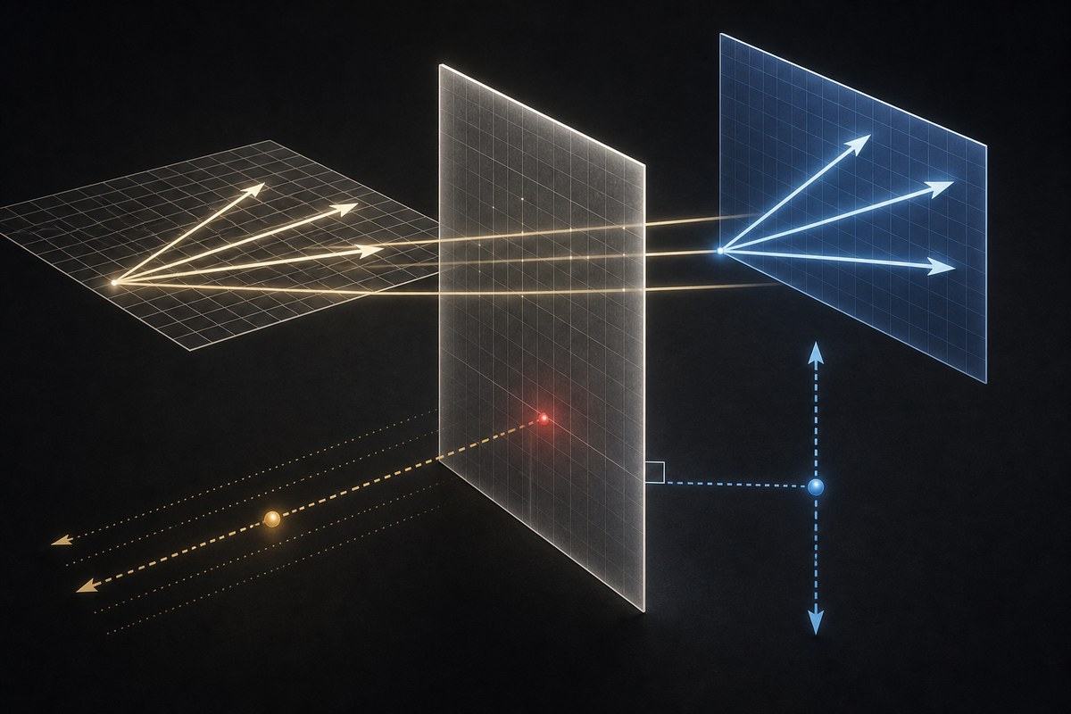
$A = \begin{bmatrix} a_{11} & a_{12} & \cdots & a_{1n} \\ a_{21} & a_{22} & \cdots & a_{2n} \\ \vdots & \vdots & \ddots & \vdots \\ a_{m1} & a_{m2} & \cdots & a_{mn} \end{bmatrix}$

Matrices represent linear transformations. When you multiply a matrix A by a vector x, you get a new vector y = *A*x. This new vector is the result of transforming x according to the rules encoded in A.

What kind of transformation? It depends on A.

Scaling: A diagonal matrix stretches or shrinks along each axis independently.
Rotation: An orthogonal matrix with determinant 1 rotates space around the origin.
Reflection: An orthogonal matrix with determinant -1 flips space across a hyperplane.
Projection: A symmetric, idempotent matrix (A² = A) projects vectors onto a subspace.
Shear: A triangular matrix slides layers of space past each other.

Any linear transformation can be decomposed into combinations of these basic operations. This is the geometric meaning of matrix decomposition, which we will discuss shortly.

Matrix multiplication is the composition of linear transformations. If A transforms space one way and B transforms it another way, then BA transforms it by doing A first, then B. The formula for matrix multiplication is:

$(AB)_{ij} = \sum_{k=1}^{n} A_{ik} B_{kj}$

That is: the entry in row i, column j of the product is the dot product of row i of A with column j of B.

Matrix multiplication is not commutative: AB ≠ BA in general. This is crucial. The order of transformations matters. Rotate then scale is not the same as scale then rotate. This non-commutativity is reflected in the non-commutativity of matrix multiplication and has profound implications for the training of neural networks, where the order of layer operations determines the representational capacity of the network.

In machine learning, matrix multiplication is the fundamental operation. A neural network layer computes y = *W*x + b, where W is a weight matrix, x is the input vector, b is a bias vector, and y is the output vector. This is a matrix multiplication followed by vector addition. A multi-layer network computes y = W₂σ(W₁x + b₁) + b₂, where σ is a nonlinear activation function. The forward pass is a sequence of matrix multiplications and nonlinearities. The backward pass (backpropagation) involves computing gradients—vectors and matrices of partial derivatives—and updating the weight matrices accordingly.

Circle Three: The Four Fundamental Subspaces

Every matrix A has associated with it four fundamental subspaces—special vector spaces that reveal the structure of the linear transformation represented by A.

The Column Space (Range): The set of all possible outputs y = *A*x. It is the subspace of the codomain that is actually reachable by the transformation. If A is an m × n matrix, the column space is a subspace of R^m. Its dimension is the rank of A.

The Null Space (Kernel): The set of all inputs x such that *A*x = 0. These are the vectors that get mapped to zero—compressed out of existence by the transformation. Its dimension is n − rank(A), by the rank-nullity theorem.

The Row Space: The column space of Aᵀ (the transpose of A). It is a subspace of R^n, orthogonal to the null space.

The Left Null Space: The null space of Aᵀ. It is a subspace of R^m, orthogonal to the column space.

These four subspaces are the skeleton of linear algebra. They tell us what a matrix does: what it can produce (column space), what it destroys (null space), what combinations of inputs matter (row space), and what constraints exist on the outputs (left null space).

In machine learning, these concepts appear in various guises:

Rank deficiency (a matrix with less than full rank) means the transformation collapses some dimensions. This can cause problems in optimization (singular Hessians) and in data analysis (multicollinearity).
The null space is related to the concept of identifiability in statistical models—if two different parameter settings produce the same output, they differ by an element of the null space.
Orthogonality between row space and null space is related to the bias-variance tradeoff in machine learning: the row space captures the signal (the directions in which the data varies), while the null space captures the noise (the directions in which the data does not vary, but where overfitting can occur).

Circle Four: Eigenvalues, Eigenvectors, and Spectral Theory

This is where linear algebra becomes truly powerful, truly beautiful, and truly essential for understanding the deep structure of matrices and the systems they represent.

An eigenvector of a matrix A is a nonzero vector v such that:

$A\mathbf{v} = \lambda \mathbf{v}$

The vector v is special: when A acts on it, v does not change direction. It is only scaled by a factor λ, which is called the eigenvalue.

Eigenvectors are the “natural directions” of a linear transformation. They are the axes along which the transformation acts purely by stretching or shrinking, without rotation or shearing. A matrix may have many eigenvectors (up to n for an n × n matrix), and they form a basis for the space if the matrix is diagonalizable.

The characteristic equation for finding eigenvalues is:

$\det(A - \lambda I) = 0$

where I is the identity matrix and det is the determinant. This is a polynomial equation in λ of degree n, so an n × n matrix has n eigenvalues (counting multiplicities and complex values).

Why do eigenvalues matter in machine learning?

Principal Component Analysis (PCA): PCA finds the eigenvectors of the covariance matrix of the data. These eigenvectors are the principal components—the directions of maximum variance. The corresponding eigenvalues tell you how much variance is captured by each component. By projecting data onto the top k eigenvectors, you reduce dimensionality while preserving as much information as possible.
Spectral Clustering: This clustering method uses the eigenvectors of a graph’s Laplacian matrix (a matrix derived from the adjacency matrix) to find communities in networks. The eigenvectors reveal the underlying structure of the graph.
PageRank: Google’s original ranking algorithm models the web as a matrix where entry (i, j) represents the probability of moving from page j to page i. The PageRank scores are the entries of the principal eigenvector (the eigenvector with eigenvalue 1) of this transition matrix.
Stability Analysis: In dynamical systems and neural networks, the eigenvalues of the Jacobian matrix (the matrix of partial derivatives) determine stability. If all eigenvalues have negative real parts, the system is stable. If any eigenvalue has a positive real part, the system is unstable. This is crucial for understanding whether a neural network will converge during training or explode/vanish.
Normalizing Flows and Diffusion Models: These generative models use linear transformations whose eigenvalue structure ensures invertibility and stable training.

Spectral Theorem: For a symmetric matrix (A = Aᵀ), the spectral theorem states that all eigenvalues are real, and the eigenvectors form an orthonormal basis. This means any symmetric matrix can be decomposed as:

$A = Q \Lambda Q^T$

where Q is an orthogonal matrix (its columns are the orthonormal eigenvectors) and Λ is a diagonal matrix (its entries are the eigenvalues). This is called eigendecomposition or spectral decomposition.

The spectral theorem is one of the most important results in linear algebra because it tells us that symmetric matrices are, in a sense, simple: they just stretch space along orthogonal axes. Many matrices in machine learning are symmetric or can be made symmetric (covariance matrices, Hessian matrices, graph Laplacians), so the spectral theorem applies directly.

Circle Five: The Singular Value Decomposition (SVD)

If eigendecomposition is the crown jewel of symmetric matrices, the Singular Value Decomposition (SVD) is the universal tool that applies to any matrix, symmetric or not, square or rectangular, full rank or rank-deficient.

The SVD states that any m × n matrix A can be decomposed as:

$A = U \Sigma V^T$

where:

U is an m × m orthogonal matrix (its columns are the left singular vectors)
Σ is an m × n diagonal matrix (its diagonal entries are the singular values, non-negative and ordered from largest to smallest)
V is an n × n orthogonal matrix (its columns are the right singular vectors)

The singular values are the square roots of the eigenvalues of AᵀA (or AAᵀ). The left singular vectors are the eigenvectors of AAᵀ. The right singular vectors are the eigenvectors of AᵀA.

Why is SVD the most important matrix decomposition in machine learning?

Dimensionality Reduction: By keeping only the top k singular values and their corresponding singular vectors, you obtain the best rank-k approximation of A in terms of the Frobenius norm. This is the mathematical foundation of Latent Semantic Analysis (LSA) for text, recommender systems (matrix factorization), and image compression.
Pseudoinverse: The Moore-Penrose pseudoinverse A⁺, which generalizes matrix inversion to non-square and singular matrices, is computed via SVD: A⁺ = V Σ⁺ Uᵀ. This is used in linear regression, least squares problems, and control theory.
Noise Reduction: In data analysis, small singular values often correspond to noise. By truncating them, you can denoise data while preserving the important structure.
Low-Rank Approximation: Many matrices in machine learning are approximately low-rank. SVD reveals this structure explicitly, allowing efficient storage and computation.
Interpretability: The singular vectors often have semantic meaning. In LSA, the left singular vectors correspond to document topics, and the right singular vectors correspond to word topics. In collaborative filtering, the singular vectors correspond to user types and item types.

Circle Six: Tensors and the Generalization to Higher Dimensions

Matrices are 2-dimensional arrays. Tensors generalize this to any number of dimensions.

A scalar is a 0-dimensional tensor (a single number).
A vector is a 1-dimensional tensor (a list of numbers).
A matrix is a 2-dimensional tensor (a grid of numbers).
A 3D tensor is a cube of numbers (e.g., a color image: height × width × channels).
A 4D tensor might be a batch of color images: batch_size × height × width × channels.
A 5D tensor might be a batch of video frames: batch_size × time × height × width × channels.

In deep learning, tensors are the fundamental data structure. Every input, every weight, every activation, every gradient is a tensor. The operations of deep learning—convolution, matrix multiplication, batch normalization, attention—are all tensor operations.

Tensor contraction generalizes matrix multiplication. Just as matrix multiplication sums over one index (the inner dimension), tensor contraction can sum over multiple indices, combining tensors of arbitrary dimensionality.

Tensor decomposition generalizes matrix decomposition. The CP decomposition (Candecomp/Parafac) decomposes a tensor into a sum of rank-1 tensors. The Tucker decomposition generalizes SVD to higher dimensions. These decompositions are used in tensor networks for quantum computing simulations, in neural network compression (decomposing weight tensors into smaller factors), and in multiway data analysis.

The mathematics of tensors is more complex than that of matrices. Not all tensors can be diagonalized. The rank of a tensor is not always well-defined. But the conceptual framework—multidimensional arrays with linear operations—extends the power of linear algebra into the high-dimensional spaces where modern machine learning operates.

Circle Seven: The Calculus of Linear Algebra—Gradients, Jacobians, and Hessians

Machine learning is not just linear algebra. It is linear algebra married to calculus, specifically multivariable calculus and optimization.

When we train a neural network, we define a loss function L that measures how badly the network is performing. The loss depends on the network’s parameters (the weights and biases, collectively denoted θ). We want to find the parameters that minimize the loss.

Gradient descent is the algorithm: start with random parameters, compute the gradient of the loss with respect to the parameters (the vector of partial derivatives), and move in the opposite direction.

$\theta_{new} = \theta_{old} - \eta \nabla_\theta L$

where η is the learning rate.

The gradient ∇_θ L is a vector. It lives in the same space as the parameters. It points in the direction of steepest ascent of the loss function, so we move in the opposite direction to descend.

For a single layer, the gradient is computed using the chain rule. If y = *W*x + b, and the loss depends on y, then:

$\frac{\partial L}{\partial W} = \frac{\partial L}{\partial \mathbf{y}} \mathbf{x}^T$

The gradient with respect to the weight matrix is the outer product of the upstream gradient (how much the loss changes with respect to the output) and the input vector. This is a rank-1 matrix update.

The Jacobian matrix generalizes the gradient to vector-valued functions. If f: R^n → R^m, the Jacobian J is the m × n matrix of all first-order partial derivatives:

$J_{ij} = \frac{\partial f_i}{\partial x_j}$

The Jacobian describes how a function locally transforms space. Its determinant (when m = n) describes how volumes are scaled. In normalizing flows—a class of generative models—the Jacobian determinant is used to compute the change of variables formula for probability densities.

The Hessian matrix is the matrix of second-order partial derivatives:

$H_{ij} = \frac{\partial^2 L}{\partial \theta_i \partial \theta_j}$

The Hessian describes the curvature of the loss landscape. Its eigenvalues determine the local geometry of optimization: large eigenvalues mean steep curvature (fast convergence but possible instability), small eigenvalues mean flat curvature (slow convergence). The condition number of the Hessian (ratio of largest to smallest eigenvalue) determines how ill-conditioned the optimization problem is.

Second-order optimization methods (Newton’s method, natural gradient) use the Hessian or its approximations to converge faster than first-order gradient descent. But computing and inverting the Hessian is expensive for large neural networks (it has O(n²) parameters and O(n³) inversion cost, where n is the number of parameters, which can be billions). This is why first-order methods like stochastic gradient descent, Adam, and RMSprop dominate deep learning, despite their slower convergence—they are computationally tractable.

Circle Eight: The Electron Level—How Computers Actually Do This

Let us descend to the hardware level, to the silicon and the electrons, because understanding how linear algebra is actually executed on physical machines illuminates why certain algorithms are preferred, why GPUs are essential for deep learning, and why the field has evolved in the directions it has.

Floating-Point Arithmetic. Computers represent real numbers using floating-point notation: a sign bit, an exponent, and a mantissa (significand). A 32-bit single-precision float (FP32) provides about 7 decimal digits of precision. A 64-bit double-precision float (FP64) provides about 16 digits. A 16-bit half-precision float (FP16) provides about 3-4 digits.

In deep learning, mixed-precision training uses FP16 for most computations (reducing memory usage and increasing speed) and FP32 for critical accumulations (preventing rounding errors from accumulating). Recent developments include bfloat16 (brain float, 16 bits with a wider range than FP16) and FP8 (8-bit floats) for even greater efficiency.

Why does precision matter? Because matrix multiplication involves billions of operations, and rounding errors accumulate. If the condition number of a matrix is large (meaning it is close to singular), small errors in the input can cause large errors in the output. This is numerical instability, and it is a constant concern in machine learning.

Memory Hierarchy and Cache. Computers have a hierarchy of memory: registers (fastest, smallest), L1/L2/L3 cache, main memory (RAM), and disk (slowest, largest). Matrix multiplication is memory-bound—the bottleneck is often not the arithmetic operations but the time spent fetching data from memory.

Tiling (or blocking) is the technique of breaking large matrices into small blocks that fit in cache, computing on each block, and moving to the next. The BLAS (Basic Linear Algebra Subprograms) library implements highly optimized tiled matrix multiplication. LAPACK builds on BLAS to provide higher-level decompositions (SVD, eigendecomposition, QR).

GPUs and Parallelism. A CPU has a few powerful cores (8–64 in modern processors) optimized for sequential tasks. A GPU has thousands of simpler cores (10,000+ in modern NVIDIA GPUs) optimized for parallel tasks. Matrix multiplication is embarrassingly parallel—each entry of the output matrix can be computed independently as the dot product of a row and a column.

GPUs are designed for graphics, which is essentially a massive parallel matrix operation (transforming 3D coordinates into 2D screen coordinates, applying texture maps, computing lighting). It turns out that the same parallel architecture is perfect for neural network training, where millions of matrix entries need to be updated simultaneously.

CUDA (Compute Unified Device Architecture) is NVIDIA’s platform for programming GPUs. cuBLAS is NVIDIA’s GPU-accelerated BLAS library. cuDNN provides GPU-optimized primitives for deep learning (convolution, pooling, activation functions). When you train a neural network in PyTorch or TensorFlow, the heavy lifting is done by these libraries, which are essentially highly optimized linear algebra engines running on massively parallel hardware.

TPUs (Tensor Processing Units) are Google’s custom ASICs (application-specific integrated circuits) designed specifically for matrix operations. They use systolic arrays—grids of processing elements that pass data rhythmically, like a heartbeat, performing matrix multiplications with extreme efficiency. A single TPU pod can perform 100+ petaflops (10¹⁵ floating-point operations per second) of matrix operations.

Distributed Training. Modern large language models (GPT-4, Claude, Gemini) have hundreds of billions of parameters. They cannot fit on a single GPU. Model parallelism splits the model across multiple devices: different layers on different GPUs, or even different parts of a single layer. Data parallelism replicates the model on multiple devices and splits the data batch across them, aggregating gradients. Pipeline parallelism combines both approaches.

All of this distributed computation is, at its core, the coordination of massive matrix operations across clusters of machines. The all-reduce operation, which aggregates gradients from multiple workers, is a collective communication primitive that is essentially a distributed matrix summation.

Quantization and Sparsity. To deploy large models on edge devices (phones, IoT sensors), we use quantization (reducing precision from FP32 to INT8 or even INT4) and sparsity (pruning small weights to zero, creating sparse matrices that can be stored and multiplied more efficiently). Sparse matrix formats (CSR, CSC, COO) and sparse matrix algorithms are active areas of research, bridging linear algebra and computer architecture.

Which Technologies, Systems, Methods, and Discoveries Make It Possible? The Infrastructure of Abstraction

Linear algebra did not become the language of machine learning by accident. It required a vast infrastructure—mathematical, computational, and cultural—to make it possible. Let me survey this infrastructure.

The Mathematical Infrastructure

Axiomatic Vector Spaces. Peano’s axioms (1888) and the subsequent development of abstract algebra by Emmy Noether and others provided the rigorous foundation. Without this axiomatic framework, we would not have the general theorems that apply across all vector spaces, finite and infinite, real and complex, Euclidean and Hilbert.

Functional Analysis. The extension of linear algebra to infinite dimensions—Hilbert spaces, Banach spaces, operator theory—provided the tools for analyzing continuous systems (differential equations, quantum mechanics, signal processing) and for understanding the limits of finite approximations.

Numerical Analysis. The development of algorithms that are both efficient (low computational complexity) and stable (robust to rounding errors) was essential. Gene Golub’s work on the SVD, the QR algorithm for eigenvalues, and iterative methods for large sparse systems transformed linear algebra from a theoretical discipline into a practical engineering tool.

The Computational Infrastructure

BLAS and LAPACK. These libraries, developed in the 1970s–1990s, standardized and optimized basic linear algebra operations. They are the foundation upon which all higher-level scientific computing is built. When NumPy performs a matrix multiplication, it calls BLAS. When SciPy computes an SVD, it calls LAPACK.

MATLAB (1984). Cleve Moler’s MATLAB (Matrix Laboratory) made matrix operations accessible to engineers and scientists without requiring them to write low-level Fortran or C. Its interactive environment and visualization tools democratized linear algebra.

Python and NumPy (2006). Travis Oliphant’s NumPy brought MATLAB-style array computing to Python, the language that would become the lingua franca of machine learning. NumPy’s ndarray object is a multi-dimensional tensor, and its broadcasting rules generalize matrix operations to arrays of different shapes.

CUDA and cuDNN (2007, 2014). NVIDIA’s CUDA platform allowed general-purpose computing on GPUs, and cuDNN provided optimized primitives for deep learning. This hardware-software co-evolution was the enabling technology for the deep learning revolution. Without GPUs, training deep networks would take months or years instead of days or hours.

Automatic Differentiation (Autograd, 2014; PyTorch, 2016; JAX, 2018). These frameworks automatically compute gradients through computational graphs, eliminating the need to manually derive and implement backpropagation. They use reverse-mode automatic differentiation, which computes the gradient of a scalar loss with respect to all parameters in a single backward pass, at a cost proportional to the forward pass. This is a linear algebraic miracle: the chain rule, applied systematically through the graph, yields the exact gradient vector without symbolic differentiation or finite differences.

Distributed Computing Frameworks (Horovod, DeepSpeed, FSDP, 2018–2022). These frameworks handle the complexity of training models across hundreds or thousands of GPUs, managing data parallelism, model parallelism, and pipeline parallelism. They are essentially distributed linear algebra schedulers.

The Algorithmic Infrastructure

The Perceptron (Rosenblatt, 1957). The first learning algorithm, a linear classifier. It proved that a machine could learn from data, though its limitations (it could not learn the XOR function, as Minsky and Papert showed in 1969) led to the first AI winter.

Backpropagation (Werbos, 1974; Rumelhart et al., 1986). The algorithm that made multi-layer neural networks trainable. It uses the chain rule to compute gradients through the network, and those gradients are vectors and matrices of partial derivatives. Backpropagation is linear algebra in action: the forward pass computes a composition of linear transformations and nonlinearities, and the backward pass computes the adjoint (transpose) of those linear transformations, propagating error signals backward through the network.

Convolutional Neural Networks (LeCun et al., 1989, 1998). CNNs use convolution—a linear operation where a small matrix (the filter) slides across a larger matrix (the image)—to detect local features. Weight sharing (the same filter applied across the image) reduces parameters and encodes translational invariance. The success of AlexNet (2012) proved that deep CNNs, trained on large datasets with GPU acceleration, could achieve superhuman performance on image recognition.

Word Embeddings (Mikolov et al., 2013). Word2Vec and GloVe showed that words could be represented as dense vectors in a semantic space, where geometric relationships encode linguistic relationships. This was a triumph of linear algebra: meaning became geometry.

Attention and Transformers (Vaswani et al., 2017). The “Attention Is All You Need” paper introduced the Transformer architecture, which replaced recurrent connections with self-attention mechanisms. Attention computes a weighted sum of value vectors, where the weights are determined by the dot product similarity between query and key vectors. It is pure linear algebra: matrix multiplications, softmax normalization (a nonlinear operation), and linear projections. Transformers are now the dominant architecture in NLP, computer vision, and multimodal AI.

Diffusion Models (Ho et al., 2020; Song et al., 2020). These generative models learn to reverse a diffusion process that gradually adds noise to data. The reverse process is parameterized by neural networks that predict noise vectors, and the sampling process involves iterative denoising in a high-dimensional vector space. The mathematics involves stochastic differential equations and score matching, but the implementation is matrix operations at scale.

The Cultural Infrastructure

Open Source. The machine learning community’s commitment to open source—PyTorch, TensorFlow, JAX, Hugging Face, and countless models and datasets released publicly—has accelerated progress by orders of magnitude. Linear algebra code that once took weeks to write and debug is now a single import statement.

Pretraining and Transfer Learning. The realization that models trained on massive, general datasets could be fine-tuned for specific tasks (BERT, GPT) changed the economics of AI. Instead of training from scratch, practitioners download pretrained weight matrices (billions of numbers) and adapt them. These weight matrices are the crystallized linear algebra of millions of hours of GPU computation.

The AI Research Community. Conferences (NeurIPS, ICML, ICLR), preprint servers (arXiv), and social media (Twitter/X, Reddit, Discord) create a global, real-time conversation. Ideas propagate at the speed of light. A new linear algebraic technique—say, a more efficient attention mechanism, or a new matrix decomposition for model compression—can be published, implemented, and adopted by the entire community within weeks.

Common Misconceptions, Limitations, and Unresolved Questions

No honest treatment of a subject is complete without acknowledging its boundaries, its blind spots, its unresolved tensions. Linear algebra is powerful, but it is not omnipotent. Let me address some common misconceptions and open questions.

Misconception 1: “Linear Algebra Is Just About Matrices and Determinants”

This is like saying literature is just about alphabet letters. Matrices and determinants are tools, not the essence. The essence is structure—the axioms of vector spaces, the properties of linear transformations, the interplay between algebra and geometry. Matrices are one representation of linear transformations, convenient for computation but not fundamental. A linear transformation exists independently of any matrix representation; the matrix is just its coordinate expression in a particular basis.

Misconception 2: “Linear Algebra Is Only for Continuous Data”

While linear algebra is most natural for real and complex vector spaces, it generalizes to discrete and finite settings. Linear codes in coding theory use vector spaces over finite fields. Graph theory uses the adjacency matrix and Laplacian matrix, which are linear algebraic objects. Combinatorics uses linear algebra to count and enumerate. The Boolean satisfiability problem can be approached using linear algebra over finite fields. The boundaries between continuous and discrete are more porous than they appear.

Misconception 3: “Deep Learning Has Made Linear Algebra Obsolete”

The opposite is true. Deep learning has made linear algebra more important, not less. Every neural network is a composition of linear transformations and nonlinear activations. The nonlinearities provide expressiveness, but the linear transformations provide the representational capacity. The weights—the parameters learned during training—are matrices and vectors. The activations are vectors. The gradients are vectors. The entire edifice is linear algebra with nonlinear frosting.

Limitation 1: Linearity Is a Local Approximation

Linear algebra studies linear systems, but the world is mostly nonlinear. A pendulum’s motion is nonlinear. Weather is nonlinear. The stock market is nonlinear. Human cognition is nonlinear. Linear algebra provides local approximations—tangent spaces, linearizations, first-order expansions—but it cannot capture global nonlinear behavior without help.

This is why machine learning uses nonlinear activation functions (ReLU, sigmoid, tanh, GELU, Swish) between linear layers. The linear layers provide the structure; the nonlinearities provide the flexibility. The universal approximation theorem tells us that a sufficiently large neural network with nonlinear activations can approximate any continuous function. But the approximation is built from linear pieces glued together by nonlinear switches.

Limitation 2: The Curse of Dimensionality

Linear algebra works in any finite dimension, but high-dimensional spaces behave counterintuitively. In high dimensions, volumes concentrate near the boundaries. Random vectors are nearly orthogonal. The nearest neighbor concept becomes fragile. The data required to sample a high-dimensional space grows exponentially.

This is the curse of dimensionality, and it is a fundamental challenge for machine learning. Linear algebra gives us the tools to operate in high-dimensional spaces, but it does not solve the problem that those spaces are mostly empty, mostly uninformative, mostly a void where data is sparse and distance metrics become meaningless.

Techniques like dimensionality reduction (PCA, t-SNE, UMAP) and manifold learning attempt to find low-dimensional structures within high-dimensional data. But these are partial solutions, heuristics, approximations. The fundamental tension remains: linear algebra gives us the machinery to operate in n dimensions, but it does not give us the data to fill those dimensions meaningfully.

Limitation 3: Computational Cost

Matrix multiplication has a time complexity of O(n³) for naive algorithms, or O(n²·³⁷³) for the fastest known theoretical algorithm (Coppersmith-Winograd and its descendants, though these are not practical). For large matrices—billions of parameters in modern language models—this is expensive.

Approximate matrix multiplication, randomized algorithms, sketching techniques, and low-rank approximations are active research areas that trade accuracy for speed. But the fundamental cost of linear algebraic operations remains a bottleneck, driving research into more efficient architectures (sparse attention, mixture of experts, state space models) that reduce the amount of matrix computation required.

Unresolved Question 1: Why Does Deep Learning Work?

This is the elephant in the room, the question that haunts every machine learning researcher. We know how deep learning works—gradient descent, backpropagation, matrix multiplications—but we do not fully know why it works. Why can a network with billions of parameters, trained on internet text, generate coherent poetry, solve logic puzzles, and write code? Why does the geometry of high-dimensional vector spaces, organized by gradient descent, produce intelligence-like behavior?

There are theories: the lottery ticket hypothesis suggests that large networks contain small subnetworks that are responsible for most of the performance; implicit regularization suggests that gradient descent prefers simple solutions; neural tangent kernels show that wide networks behave like kernel methods in certain limits. But none of these theories is complete. The question remains open, and it is fundamentally a question about the geometry of high-dimensional spaces—the domain of linear algebra.

Unresolved Question 2: What Is the Right Geometry for Intelligence?

Euclidean vector spaces are the default setting for machine learning, but they may not be the right geometry for intelligence. Riemannian geometry (curved spaces) might be more appropriate for representing hierarchical structure. Hyperbolic spaces (negatively curved) have been shown to embed trees and hierarchies more efficiently than Euclidean spaces. Symmetric spaces and Lie groups appear in robotics and computer vision. Information geometry uses the Fisher metric to define a Riemannian structure on the space of probability distributions.

The future of machine learning may involve moving beyond flat vector spaces to more sophisticated geometric structures, and linear algebra will be the ladder we use to climb into those higher geometries.

Unresolved Question 3: Can We Make Linear Algebra More Biologically Plausible?

The brain does not perform backpropagation. It does not compute exact gradients. It does not store weight matrices in the way artificial neural networks do. Yet it learns, adapts, and exhibits intelligence. Neuromorphic computing attempts to build hardware that mimics biological neural networks, using spike-based computation rather than matrix multiplication. Local learning rules (Hebbian learning, contrastive Hebbian learning) update synapses based on local activity without global error signals.

Can we build intelligent systems that do not rely on massive matrix operations? Or is matrix multiplication so fundamental to information processing that any sufficiently complex learning system will converge upon it, whether biological or artificial? This is an open question at the intersection of linear algebra, neuroscience, and philosophy.

The Bigger Picture: Where This Leaves Us

I began this journey by confessing that I did not choose to care about linear algebra.

I suspect you did not either.

Most of us come to this subject through necessity, through the side door, through the realization that something we want to understand—machine learning, quantum computing, computer graphics, data science—requires a fluency in a language we never learned to speak.

But here is what I have come to believe, after years of wandering through vector spaces and matrix decompositions, after watching neural networks learn and fail and learn again, after seeing the same mathematical structures appear in physics and linguistics and finance and biology:

Linear algebra is not just a tool.

It is a way of seeing.

When you understand linear algebra, you begin to see structure everywhere. You see a dataset not as a collection of rows and columns but as a cloud of points in a high-dimensional space, waiting to be rotated, projected, compressed, and understood. You see a neural network not as a black box but as a sequence of linear transformations carving pathways through vector space, bending and folding the geometry of representation until the categories emerge, clean and separable, from the chaos of raw data. You see a language model not as a chatbot but as a vast, high-dimensional embedding space where words are vectors and meaning is distance and analogy is vector arithmetic.

You see the world as a space of possibilities, and linear algebra as the grammar that allows you to navigate that space.

This is why the history matters. When you know that Chinese mathematicians were performing Gaussian elimination two thousand years ago, that Grassmann’s abstract vector spaces were dismissed as incomprehensible in his lifetime, that Cayley invented matrix algebra as a purely theoretical exercise before anyone knew what a computer was—you understand that mathematics is not a fixed edifice but a living conversation across centuries. Every theorem is a response to a question asked by someone long dead. Every algorithm is a descendant of an idea that germinated in a different world.

This is why the mechanisms matter. When you understand that a matrix multiplication is a composition of linear transformations, that an eigenvector is a direction preserved by transformation, that the SVD decomposes any matrix into a rotation, a scaling, and another rotation—you stop seeing linear algebra as a collection of recipes and start seeing it as a unified theory of structure and change.

This is why the applications matter. When you realize that the same mathematics describes the vibrations of a bridge, the quantum states of an electron, the semantic relationships between words, and the hidden layers of a neural network—you glimpse something profound about the unity of knowledge. The universe, it seems, speaks in vectors. And linear algebra is the dictionary.

But I want to end not with grandeur but with humility.

Linear algebra is powerful, but it is not complete. It describes linear structures in a world that is mostly nonlinear. It operates in finite dimensions while the universe may be infinite. It assumes exact arithmetic while computers deal in approximations. It is a map, not the territory—a beautifully precise, enormously useful map, but a map nonetheless.

The future of machine learning will likely require geometries beyond Euclidean vector spaces: curved manifolds, discrete graphs, probabilistic spaces, quantum Hilbert spaces. It will require algebras beyond matrices: tensors, operators, categories. It will require us to think not just about static structures but about dynamic processes, not just about spaces but about flows through spaces, not just about linearity but about the creative, generative power of nonlinearity.

But whatever comes next, it will build upon linear algebra. It will use linear algebra as its foundation, its scaffolding, its native tongue. Because linear algebra is not just the hidden architecture of machine learning. It is one of the hidden architectures of thought itself—the way we organize complexity, the way we find patterns in chaos, the way we make the abstract concrete and the concrete abstract.

I did not choose to care about linear algebra.

But I am glad I learned to.

And I hope, if you have read this far, that you are beginning to care too.

Not because you have to.

But because you see, now, what was always there, beneath the surface, behind the screen, inside the matrix: a structure of breathtaking elegance, a language of universal reach, a quiet tyrant that rules not by force but by the irresistible logic of its own internal beauty.

The vectors are waiting.

The matrices are multiplying.

The spaces are opening.

Step inside.

P.S. References and Further Reading

For those who wish to continue this journey, here are some resources that have shaped my understanding:

Textbooks:

Linear Algebra Done Right by Sheldon Axler — The clearest, most elegant introduction to the abstract theory.
Introduction to Linear Algebra by Gilbert Strang — The classic, with Strang’s inimitable warmth and geometric intuition.
Matrix Computations by Gene Golub and Charles Van Loan — The bible of numerical linear algebra.
Deep Learning by Ian Goodfellow, Yoshua Bengio, and Aaron Courville — The foundational text, with extensive linear algebraic foundations.
Mathematics for Machine Learning by Marc Peter Deisenroth, A. Aldo Faisal, and Cheng Soon Ong — A modern, comprehensive treatment.

Online Resources:

Gilbert Strang’s MIT OpenCourseWare lectures on Linear Algebra — freely available and genuinely wonderful.
3Blue1Brown’s “Essence of Linear Algebra” series on YouTube — visual, intuitive, beautiful.
The Matrix Calculus You Need For Deep Learning by Terence Parr and Jeremy Howard — a focused, practical guide.

Papers:

Vaswani et al., “Attention Is All You Need” (2017) — The Transformer architecture, pure linear algebra.
Mikolov et al., “Efficient Estimation of Word Representations in Vector Space” (2013) — Word2Vec and the geometry of language.
Rumelhart et al., “Learning Representations by Back-Propagating Errors” (1986) — The paper that made deep learning possible.

Historical:

The History of Linear Algebra by various authors — scattered across mathematical histories, with Grassmann’s story particularly poignant.
The Nine Chapters on the Mathematical Art — translated by Shen Kangshen, John Crossley, and Anthony Lun — for the ancient Chinese roots.

Word Cloud

Related reading