The Equation That Eats Its Own Tail: A Story of Differential Equations
On this page
Uses the speech voice supplied by your browser or device.

The Equation That Eats Its Own Tail
Prologue: The Leaky Bathtub
Imagine you are staring at a bathtub. The faucet is running, but the drain is open. The water level is doing something interesting: it depends on how much water is already in the tub. More water means a greater pressure head above the drain, which usually means that water escapes faster. Meanwhile, the faucet pours in at a constant rate, with the serene indifference of a municipal employee nearing lunch.
Let be the depth of the water. If the tub has cross-sectional area , conservation of water gives us:
The left-hand side is the rate at which the amount of water in the tub changes. The right-hand side is what enters minus what leaves.
For an idealized small opening, the outflow often grows roughly like the square root of the water depth:
so the equation becomes:
If the tub is nearly empty, the drain is feeble and the water level rises. If the water is deep, the drain becomes more enthusiastic. Eventually the inflow and outflow may balance, and the water settles at an equilibrium depth.
Now here is the slightly unsettling part: the present water level determines the rate at which the water level changes, and that rate produces the next water level, which determines the next rate, which produces the next level, and so on.
The state creates the slope. The slope creates the next state.
The bathtub is eating its own tail.
This is the essential weirdness—and the essential power—of a differential equation.
Part I: What These Things Actually Are
Most equations you met in school were like snapshots. asks: what number, when added to three, gives seven? It is a photograph of a balance scale. The answer is a number. You find it, you circle it, you move on.
A differential equation is not a photograph. It is a movie.
It does not merely ask, “What is the value?” It asks, “How is the value changing, and what does that change depend on?”
Formally, an ordinary differential equation, or ODE, relates an unknown function of one independent variable to one or more of its derivatives. If is some quantity—position, temperature, money in a bank account, the number of bacteria in a flask—then an ODE might say:
In plain English: the rate at which changes is proportional to itself.
When , this can describe idealized population growth or continuously compounded interest. When , it describes exponential decay, such as the decline of a radioactive substance. The larger the present quantity, the larger the magnitude of the change.
A partial differential equation, or PDE, extends the idea to a function that depends on several independent variables. Instead of , we might have : the temperature at position and time .
The one-dimensional heat equation is:
The left side asks how the temperature at a point is changing with time. The right side measures the local curvature of the temperature profile in space.
If a point is hotter than its immediate surroundings, that local peak tends to flatten. If it is colder, the dip tends to fill in. It is social conformity written in calculus, although the molecules have neither committees nor minutes.
In several spatial dimensions, the same equation is written:
where , the Laplacian, measures spatial curvature in every direction available.
The Equation Is Not Enough
There is an important piece of luggage that popular explanations often leave abandoned at the station.
A differential equation does not usually determine one unique solution by itself.
Consider:
Its solutions form an entire family:
where can be any constant. The equation tells us what kinds of trajectories are allowed, but it does not tell us which trajectory our particular system occupies.
To select one, we need an initial condition. If we are told that:
then , and the solution becomes:
A second-order equation usually needs two pieces of initial information. Newton’s equation for a moving object, for example, normally requires both its initial position and its initial velocity.
PDEs are greedier. They may require an initial field, boundary conditions, or both. If you want to calculate heat flow through a metal rod, you must specify not only the heat equation but also the starting temperature and what happens at the ends of the rod. Are the ends insulated? Held at fixed temperatures? Being heated by a small but vindictive flame?
The equation supplies the possible grammar. The initial and boundary conditions tell us which sentence the physical system is actually speaking.
There is another qualification. Not every differential equation describes time.
The equation of a hanging chain describes a spatial shape. Laplace’s equation describes equilibrium fields. Geodesic equations describe paths through curved spaces. “Differential” means that the equation involves rates of change with respect to some variable, not necessarily the ticking of a clock.
Still, when time is one of the variables, differential equations become machines for producing futures from presents.
Part II: A Brief and Partial History of Change
The 17th Century: The Invention of Motion
Differential equations were not discovered like a fossil in a cliff. They were developed because people needed a language capable of describing motion without reducing it to a sequence of frozen poses.
Isaac Newton needed to explain how planets move. Not merely that they trace ellipses, as Kepler had found, but why an object continually falling toward the Sun could somehow keep missing it.
Newton’s second law is usually written:
By itself, this is a compact physical relation. It becomes a differential equation for position when acceleration is written as the second derivative of position and the force is specified as a function of position, velocity, or time:
The equation ties position to velocity, velocity to acceleration, and acceleration to force. Gravity changes the motion; the motion changes the position; the position changes gravity’s direction and strength. Another tail enters another mouth.
Gottfried Wilhelm Leibniz independently developed calculus at roughly the same historical moment and supplied much of the notation we still use. His notation made derivatives look enough like fractions to be manipulated with algebraic instinct, although they are not literally ordinary fractions in every context.
Notation matters. A good notation does not merely record thought. It makes certain thoughts easier to have.
Newton possessed enormous physical insight, but Leibniz gave calculus handwriting suitable for travel.
The 18th Century: The Bernoulli Family Business
If the seventeenth century invented the tool, the eighteenth built the workshop.
The Bernoulli family treated mathematics rather like a hereditary trade, except that instead of inheriting a bakery and arguing over the ovens, they inherited calculus and argued over priority.
In 1696, Johann Bernoulli posed the brachistochrone problem: what shape of track allows a bead, moved only by gravity, to descend between two points in the shortest possible time?
The obvious answer is a straight line.
The obvious answer is wrong.
The winning curve is a cycloid. Solutions were produced by Johann Bernoulli, Jakob Bernoulli, Leibniz, l’Hôpital, and Newton, who reportedly solved the challenge with the brisk irritation of a man whose evening had been interrupted.
The related catenary problem asked for the shape of a flexible chain hanging under its own weight. Jakob and Johann Bernoulli, Leibniz, and Christiaan Huygens helped establish that the curve was not a parabola but a hyperbolic cosine:
These problems helped produce the calculus of variations, in which one does not merely search for the best number. One searches for the best entire function or path.
Leonhard Euler then arrived and systematized nearly everything within reach. He was one of the most prolific mathematicians in history. He developed broad methods for differential equations, helped standardize notation such as , transformed the theory of exponential and trigonometric functions, and left so much mathematics behind that later generations have spent centuries sorting the furniture.
Reading Euler is like watching someone who has memorized the ocean.
The 19th Century: Heat, Light, and the Arrival of Chaos
Joseph Fourier wanted to understand heat flow. In particular, he wanted to know how temperature changed inside solid objects.
The result was the heat equation, and his method of solving it involved representing broad classes of functions as sums of sines and cosines:
The details of which functions can be represented, where the series converges, and what it converges to required considerable later care. Mathematics, like plumbing, becomes most interesting just after someone says, “It is basically obvious.”
Fourier analysis nevertheless reshaped science. It now sits beneath signal processing, audio compression, image reconstruction, telecommunications, spectroscopy, and MRI.
Meanwhile, celestial mechanics was becoming less polite.
Henri Poincaré studied the three-body problem: three masses pulling on one another through gravity. No general elementary formula exists that simply accepts three arbitrary bodies and produces their trajectories for all time.
While revising a prize-winning memoir after discovering a serious error in it, Poincaré encountered extraordinarily tangled behaviour. Trajectories could follow fixed deterministic laws while remaining violently sensitive to small differences in their starting conditions.
He did not solve the three-body problem in the old hoped-for sense. Instead, he uncovered some of the mathematical machinery of what we now call chaos.
It was rather like missing the requested bus and accidentally discovering aviation.
The 20th Century: From Physics to Everything
During the twentieth century, differential equations escaped the physics department and began turning up everywhere.
The Hodgkin–Huxley equations described the electrical activity of nerve membranes. The Kermack–McKendrick equations helped establish mathematical epidemic modelling. The Black–Scholes PDE described the theoretical pricing of certain options and related financial claims under a particular collection of assumptions.
Edward Lorenz reduced atmospheric convection to three coupled equations:
These were not a complete model of the weather. They were a drastically simplified model of convection. Yet they produced behaviour so intricate that the system became an emblem of deterministic chaos.
Then the digital computer arrived.
Closed-form solutions had always been rare. Most interesting differential equations refuse to collapse into a tidy expression involving exponentials, sines, and a small ceremonial appearance by .
Computers allowed mathematicians and scientists to approximate solutions step by step. We could stop demanding formulas and start calculating trajectories.
We could simulate.
Part III: The Zoo of Equations
Let us inspect a few inhabitants of this zoo, moving from the domesticated to the mildly unruly.
The Exponential: Growth Without Limits
Given the initial condition , the solution is:
If , the quantity grows exponentially. This can describe bacteria during the early unconstrained phase of growth, when food and space have not yet become subjects of litigation. It also describes continuously compounded interest.
If , the same equation describes exponential decay.
The lesson is simple and regularly ignored: when the rate of growth depends on the current size, you do not get linear progress. You get a ski slope attempting to become a cliff.
But pure exponential growth cannot continue forever in a finite environment. Eventually the bacteria run out of nutrients, the market runs out of customers, or the office runs out of people who have not yet been invited to the meeting.
Reality begins applying the brakes.
The Logistic: Growth With a Ceiling
The logistic equation adds one such brake:
Here, is the carrying capacity.
When is much smaller than , the factor is close to one, so the behaviour resembles exponential growth.
When approaches , the factor approaches zero, and growth slows.
For , the resulting trajectory has an S-shape: a slow beginning, a rapid middle, and a gradual approach to saturation.
This can serve as a rough model of population growth, technology adoption, or market saturation. In crude epidemic approximations, cumulative cases may resemble a logistic curve. Daily new cases correspond to its derivative, which is roughly bell-shaped rather than S-shaped.
Real epidemics are generally more complicated. Susceptibility, infection, recovery, immunity, behaviour, public policy, new variants, and reporting delays all enter the room and begin moving the furniture. Models such as SIR and its descendants use several coupled differential equations to represent these compartments.
The logistic equation is not reality. It is one useful sketch of reality behaving itself.
The Wave Equation: How Disturbances Travel
This PDE describes how disturbances propagate through many idealized systems.
Pluck a guitar string. The point you displaced is pulled back toward equilibrium, but it is coupled to nearby points, which are coupled to their neighbours. The disturbance travels down the string rather than remaining where your finger placed it.
Every point consults its immediate neighbourhood. Information moves through the system at a finite speed .
Versions of the wave equation describe vibrating strings and membranes, sound in suitable media, seismic waves, and components of electromagnetic fields in simple source-free environments. Wi-Fi does not require molecules to carry it across your room, but its electromagnetic ancestry still leads back to wave equations.
The equation is local. The wave is global.
No point on the string needs to know the shape of the entire vibration. Each point merely obeys the rule in its own small neighbourhood, and the large-scale pattern assembles itself.
The Heat Equation: The Great Averager
Again:
If a region is hotter than its surroundings, heat tends to flow outward. If it is colder, heat tends to flow inward.
Under suitable conditions—an insulated connected object with no internal heat sources, for example—the temperature eventually becomes uniform. With fixed but unequal boundary temperatures, the system instead approaches a nonuniform steady profile.
The heat equation does not always flatten everything into one temperature. It drives the system toward the equilibrium permitted by its boundaries and sources.
The same mathematical structure describes diffusion. A concentrated chemical spreads through a solvent. The probability density of a Brownian particle broadens. A sharp feature in an image can be smoothed by allowing an artificial diffusion process to run for a while.
The heat equation is a machine for sanding down gradients.
This is useful when the gradient is noise.
It is less useful when the gradient is the edge of someone’s nose.
Part IV: How the Movie Is Made One Frame at a Time
A differential equation gives us a local rule. But how does a local rule become an entire trajectory?
Suppose:
At the present point , the function tells us the slope. If we take a small time step , we can estimate the next value by moving along that slope:
This is Euler’s method.
Consult the slope. Take a small step. Consult the new slope. Take another step. Continue until you have marched from the present into the future or until the numerical calculation catches fire.
If the steps are too large, the approximation may be poor or unstable. If they are extremely small, the calculation becomes expensive. More sophisticated methods—Runge–Kutta schemes, multistep methods, symplectic integrators, implicit solvers—try to balance accuracy, stability, and computational cost.
Some solvers adjust their step sizes automatically. They take larger steps when the trajectory is smooth and smaller steps when it bends sharply or becomes numerically troublesome.
This small formula:
is one of the hidden bridges between differential equations and machine learning.
A residual neural-network layer often has the form:
Gradient descent has the form:
Both resemble Euler steps.
The modern machine-learning edifice, which regularly presents itself as a gleaming new continent, has several old differential-equation tunnels running underneath it.
Part V: The Secret Life of Differential Equations in AI
Here is where the story takes a turn that would make Fourier put down his quill and ask to see the source code.
For most of their history, differential equations were used primarily to express models of physical systems. Scientists wrote them because they believed forces, flows, fields, reactions, or populations changed according to particular local laws.
In recent years, the relationship with machine learning has become bidirectional.
Machine learning can help approximate solutions to differential equations. Differential equations can also help us understand, design, and train machine-learning systems.
Neural ODEs: Deep Learning as a Continuous Process
A standard deep neural network is a layer cake. Data enters one layer, is transformed, enters another layer, is transformed again, and continues through perhaps dozens or hundreds of stages.
A residual network writes each step as:
This looks suspiciously like Euler’s method.
In 2018, Ricky T. Q. Chen and collaborators asked what would happen if the discrete layer index were replaced by a continuous variable. Rather than specifying a finite stack of transformations, they described the hidden state with an ODE:
Here, is usually represented by a neural network with parameters . The input supplies the initial condition , and a numerical ODE solver produces the output .
The popular description is that the network has infinitely many infinitesimally thin layers. This is a useful picture, provided we remember that an actual computer still evaluates the vector field a finite number of times.
Why do this?
One reason is that continuous-time models fit naturally with data observed at irregular times. If a patient’s measurements occur at 9:03, 11:47, and three days later, a continuous model does not have to pretend that the universe works in evenly spaced spreadsheet rows.
Another reason is adaptive numerical computation. The solver can use large or small steps according to its estimate of numerical error. The solver, rather than the neural network by itself, decides how many evaluations are required to meet a chosen tolerance.
There can also be memory advantages. Adjoint-based methods can compute gradients without storing every intermediate solver state, instead reconstructing or recomputing information during the backward pass. This trades memory for additional computation and may introduce numerical difficulties. In practice, checkpointing and other gradient methods are often used when accuracy matters more than the elegance of the sales brochure.
Neural ODEs are not automatically better than ordinary residual networks. They can be slower, harder to optimize, and constrained by the behaviour of the numerical solver.
But they change the conceptual picture.
The network is no longer merely a stack of operations.
It is a learned flow through a state space.
Diffusion Models: Noise, Probability, and the Road Back
You have seen the results: systems that begin with noise and generate faces, landscapes, illustrations, rooms, animals, machinery, and cats wearing clothing they would reject if consulted.
The word diffusion tempts us into a simple story: take a clean image, blur it with the heat equation, and then run the heat equation backward.
That story is memorable.
It is also not quite right.
In a standard diffusion model, the forward process progressively adds Gaussian noise to data. The image does not merely smear into neighbouring pixels as heat spreads through a metal plate. Instead, the point representing the entire image wanders through a high-dimensional data space whose coordinates may be pixel values or latent variables.
In discrete diffusion models, noise is added through a sequence of small probabilistic steps. In continuous time, the process can be described by a stochastic differential equation:
The first term describes a systematic drift. The second adds random motion through a Wiener process, the mathematical idealization behind Brownian noise.
As time passes, the complicated distribution of real images is pushed toward a much simpler distribution, usually something close to a Gaussian cloud.
The probability density evolves according to a Fokker–Planck equation. In special cases, this has a deep relationship to a heat equation—but a heat equation in high-dimensional data space, not ordinary warmth flowing from one pixel to the next.
The reverse process requires knowledge of the score:
The score is a vector pointing in the local direction where probability density increases most sharply.
A neural network is trained to estimate this vector field:
Depending on the particular formulation, the network may be trained to predict the noise, the original clean sample, a velocity-like quantity, or the score itself. These parameterizations differ in implementation but supply the information needed to construct the reverse dynamics.
Begin with Gaussian noise. Follow the learned reverse-time stochastic process—or a related deterministic probability-flow ODE—and the noise gradually acquires structure.
Edges appear. Shapes cohere. A face emerges. Somewhere, against all reasonable odds, the cat receives a top hat.
Text conditioning bends this learned vector field toward regions compatible with the prompt.
The model has not simply learned to run ordinary heat conduction backward. The literal backward heat equation is notoriously unstable: tiny errors explode as one attempts to reconstruct lost detail.
A diffusion model instead learns how to reverse a deliberately designed stochastic noising process by using statistical information extracted from a large collection of examples.
The kinship with heat is real.
But it lives in probability space and requires a learned guide.
Physics-Informed Neural Networks: When Equations Meet Sparse Data
Suppose you know a differential equation but possess only a small number of observations. Perhaps you want to infer an unknown material parameter, reconstruct a hidden field, or combine sparse sensor readings with a physical model.
A physics-informed neural network, or PINN, represents the unknown solution with a neural network:
Automatic differentiation allows us to calculate derivatives such as:
Suppose the governing PDE can be written abstractly as:
We can define a residual:
The training loss may then combine several terms:
The network is punished for disagreeing with observations, violating the differential equation at sampled collocation points, or disobeying the initial and boundary conditions.
This can be useful, especially in inverse problems where the goal is not merely to solve a known equation but to infer unknown parameters from incomplete measurements.
But the phrase physics-informed must not be confused with physics-certified.
The equation is usually imposed as a soft penalty, not an inviolable law. A network can achieve a small residual at sampled points while remaining inaccurate elsewhere. The competing loss terms can be badly scaled. Training may become difficult for stiff equations, turbulent flows, multiscale systems, advection-dominated problems, or long-time chaotic dynamics.
For routine forward simulation, classical finite-difference, finite-volume, finite-element, or spectral solvers are often more accurate and efficient.
A PINN is not a neural replacement for all numerical physics. It is a framework for combining equations, data, and optimization, sometimes very usefully and sometimes with the confidence of a man attempting to repair a bridge using a motivational poster.
The artist has been handed the building code.
That does not yet make the building safe.
The Dynamical-Systems View of Optimization
When a neural network is trained, an optimizer adjusts its parameters to reduce a loss function.
The familiar gradient-descent update is:
This is precisely the forward-Euler form of the differential equation:
The continuous equation is called gradient flow.
The parameter vector behaves like a point sliding down a landscape whose height is the loss. The negative gradient gives the direction of steepest local descent.
The learning rate plays the role of a time step. If it is too small, training crawls. If it is too large, the optimizer may overshoot, oscillate, or launch itself into numerical outer space.
Momentum can be understood through a second-order dynamical system:
Now the parameters possess something analogous to velocity. The damping term dissipates motion, while the gradient pulls the system downhill.
Properly tuned momentum can reduce wasteful zigzagging across narrow valleys and accelerate movement in directions where the gradient remains consistent.
Poorly tuned momentum can overshoot and oscillate with considerable enthusiasm.
The dynamical-systems view has also produced rigorous results for very wide neural networks. In one analytically tractable infinite-width regime, training remains close to the network’s initialization and approaches a nearly linear kernel dynamics described by the neural tangent kernel.
This is mathematically powerful.
It is not a complete explanation of why practical finite neural networks learn useful features or generalize well. Real networks may travel far from their initial states and change their internal representations in ways that the simplest fixed-kernel picture cannot capture.
Another question concerns implicit regularization.
A large neural network may possess many different parameter settings that fit the training data. Gradient descent does not select among them uniformly. The architecture, parameterization, initialization, optimizer, step size, and trajectory all introduce biases.
In certain simplified settings, gradient-based methods can be shown to favour minimum-norm or maximum-margin solutions. In more realistic networks, the full story remains active research.
The optimizer is not merely finding a minimum.
It is finding a minimum reachable by a particular kind of journey.
Part VI: What This Is Secretly Teaching Us
Differential equations are not merely a branch of mathematics. They are a way of seeing.
They teach us that local rules can generate global behaviour.
A point on a string does not know the full wave. A parcel of fluid does not consult a map of the entire atmosphere. Each part responds to its immediate state and neighbourhood. The large-scale pattern emerges from repeated local obedience.
But the rule is not the whole story. Parameters, initial conditions, boundary conditions, and external forcing decide which of the permitted behaviours actually appears.
The equation is the seed.
The conditions decide what soil it has landed in.
Differential equations also teach us that prediction is a form of integration.
To know the future, we accumulate all the tiny changes between now and then. Numerical solvers make this literal: calculate a slope, take a step, calculate another slope, take another step.
Errors accumulate too.
In a stable system, small numerical or observational errors may remain small or die away. In a chaotic system, they can grow exponentially. The laws may be perfectly deterministic while useful long-term prediction becomes impossible.
Determinism is not the same thing as predictability.
A clock and a storm may both obey differential equations. Only one is considerate enough to keep an appointment.
They teach us that continuous and discrete descriptions are closely related but not interchangeable.
A differential equation can be approximated by discrete steps. A residual network can resemble a discretized flow. Gradient descent can be viewed as a numerical integrator.
But discretization can also introduce behaviour absent from the continuous system. The continuous logistic ODE approaches a carrying capacity smoothly. The discrete logistic map can oscillate, period-double, and become chaotic.
The two languages often translate into each other.
They do not always tell precisely the same story.
Differential equations reveal deeper structures beneath apparently different physical laws.
Many equations of mechanics can be derived from a principle of stationary action. “Stationary” does not always mean “smallest”; it means that the action does not change to first order under tiny variations of the path.
Ideal wave equations conserve an energy under appropriate boundary conditions and in the absence of damping or forcing.
Diffusion equations dissipate gradients and can often be interpreted as flows descending an energy or free-energy functional in a suitable geometry.
These are not signs that nature is lazy, nor that the universe spent billions of years optimizing its regulations after an extended consultation process.
They reveal relationships among symmetry, conservation, geometry, and dissipation. A local differential equation may be the visible surface of a deeper organizing principle.
Finally, differential equations teach a useful humility.
An equation is not nature itself.
Some equations express extraordinarily fundamental laws. Others are approximations valid only under restricted conditions. The heat equation assumes a continuum description. The logistic equation compresses ecology into one population and one ceiling. Black–Scholes relies on assumptions that real markets regularly inspect and then violate.
Every model discards something.
The question is not whether the model is perfectly true. It is whether it preserves the features that matter for the problem at hand.
An elegant equation can illuminate reality.
It can also illuminate only its own elegance.
Knowing the difference is part of the mathematics.
Part VII: A Compact Takeaway
A differential equation is a conditional promise.
For an evolution problem, it says: give me the rule, the relevant parameters, the initial state, and the boundary conditions, and I will tell you how the system attempts to step into the future.
It is not a complete map.
It is a set of walking instructions.
Sometimes the instructions produce one clear path. Sometimes several paths are possible. Sometimes the solution becomes unstable, singular, chaotic, or impossible to extend. Sometimes the numerical traveller mistakes an error in the compass for a continent.
But the central idea remains astonishingly simple.
The present state determines a local rate of change.
That rate produces the next state.
The next state determines the next rate.
The equation eats its own tail, one infinitesimal bite at a time.
From Newton’s planets to Fourier’s heat, from Hodgkin and Huxley’s nerve impulses to Lorenz’s convecting atmosphere, from residual networks to diffusion models generating an image from noise, the grammar has not fundamentally changed.
Only the sentences have grown longer.
References
Chen, R. T. Q., Rubanova, Y., Bettencourt, J., & Duvenaud, D. (2018). “Neural Ordinary Differential Equations.” Advances in Neural Information Processing Systems.
Hairer, E., Nørsett, S. P., & Wanner, G. (1993). Solving Ordinary Differential Equations I: Nonstiff Problems. Springer.
Ho, J., Jain, A., & Abbeel, P. (2020). “Denoising Diffusion Probabilistic Models.” Advances in Neural Information Processing Systems.
Jacot, A., Gabriel, F., & Hongler, C. (2018). “Neural Tangent Kernel: Convergence and Generalization in Neural Networks.” Advances in Neural Information Processing Systems.
Krishnapriyan, A., Gholami, A., Zhe, S., Kirby, R., & Mahoney, M. W. (2021). “Characterizing Possible Failure Modes in Physics-Informed Neural Networks.” Advances in Neural Information Processing Systems.
Raissi, M., Perdikaris, P., & Karniadakis, G. E. (2019). “Physics-Informed Neural Networks: A Deep Learning Framework for Solving Forward and Inverse Problems Involving Nonlinear Partial Differential Equations.” Journal of Computational Physics.
Sohl-Dickstein, J., Weiss, E. A., Maheswaranathan, N., & Ganguli, S. (2015). “Deep Unsupervised Learning Using Nonequilibrium Thermodynamics.” Proceedings of the International Conference on Machine Learning.
Song, Y., Sohl-Dickstein, J., Kingma, D. P., Kumar, A., Ermon, S., & Poole, B. (2021). “Score-Based Generative Modeling Through Stochastic Differential Equations.” International Conference on Learning Representations.
Strogatz, S. H. (2014). Nonlinear Dynamics and Chaos. Westview Press.
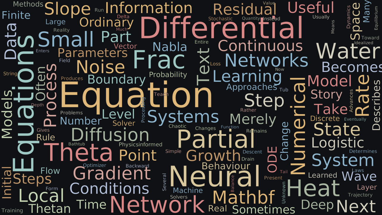
Word Cloud
Related reading
Selected by shared topics and section, with closer publication dates breaking ties.