The Bouncer, the Clock, and Big O
On this page
Uses the speech voice supplied by your browser or device.

Why Should We Care? (Or: The Nightclub of Computation)
Imagine you are trying to get into a nightclub. There are two bouncers at the door. One bouncer checks your ID, glances at the guest list, and waves you through in a few seconds. The other bouncer interrogates every person in line, compares your face to every photo on a wall of thousands, and then makes you solve a riddle before you can enter. Both bouncers get the job done, but one of them will have a very long line by midnight.
In the world of computers, time complexity describes how the waiting time grows as the crowd gets bigger. Space complexity is the size of the nightclub itself—how much room you need to store all the guests, the guest list, the riddle props, and the bouncer’s increasingly elaborate security system.
For decades, these were among the main costs computer scientists worried about. If your algorithm was fast and did not eat all the RAM, you were golden. But lately, a third bouncer has shown up. This one does not clearly explain why it makes its decisions. It just nods, and sometimes it is instant, and sometimes it takes longer, and sometimes it hallucinates your name and lets in a mannequin by mistake. This is the AI black box, and it is not abolishing the old rules of the nightclub, but it is exposing how much those rules never attempted to measure.
The Core Intuition: Counting Steps, Not Seconds
Here is the first thing to understand about algorithmic complexity: we usually do not care about seconds. We care about trends. We care about what happens when your “small” problem becomes a “medium” problem, and then a “massive” problem, and then a “we-need-to-buy-a-bigger-datacenter” problem.
If I give you a list of ten names and ask you to find “Alice,” you might just read down the list. Ten names, ten glances. Easy. If I give you a million names, you read down the list. A million glances. The work grew in direct proportion to the size of the list. We call this linear time, or . The is the number of items, and the describes an upper bound on how the work grows. It is not a scary symbol; it is a way of saying, “However many things we have, the work grows roughly in this shape.”
Now, what if the list is sorted alphabetically? You open the book in the middle. If the name in the middle starts with “M” and you are looking for “Alice,” you know she must be in the first half. You throw away the second half. You open the middle of the first half. “F”? Throw away the second half of that. You keep cutting the problem in half. For a million names, you only need about twenty glances. The work grew logarithmically. We call this . It is the mathematical equivalent of a cheat code.
Here is the beautiful, terrible truth: computers are fast, but bad algorithms are patient. A bad algorithm will wait. It will lurk. It will seem fine when you have a hundred items, and then it will eat your entire afternoon when you have ten thousand. Complexity analysis is how we spot the monster in the nursery before it grows up.
The Notation Zoo: A Gentle Field Guide
Computer scientists, being the theatrical people they are, have invented a whole family of notations to describe how algorithms behave. Think of them as different kinds of boundary fence.
Big-O: The Ceiling
says: “Beyond some sufficiently large input size, the cost will not grow faster than a constant multiple of this function.” It is an upper bound on growth.
Big-O is often used to describe worst-case running time, which is why people casually treat it as the notation of pessimism. But Big-O itself does not mean “worst case.” It can describe worst-case time, average time, memory use, network traffic, or almost any other cost we have chosen to measure. It is the ceiling of the nightclub, although we must first say which room we are measuring.
Big-Omega: The Floor
says: “The cost grows at least this quickly.” It is a lower bound.
Again, it does not automatically mean “best case.” It means that the particular cost function being discussed cannot asymptotically fall below that rate. In comparison-based sorting, for example, the worst-case number of comparisons cannot generally be better than . It is the floor of the nightclub.
Big-Theta: The Tight Fit
says: “The cost is bounded both above and below by constant multiples of this function.” It grows asymptotically like —neither fundamentally faster nor fundamentally slower.
If an algorithm takes time, then captures the shape of its growth rather tightly. It is the nightclub whose architect has measured both the floor and the ceiling and, for once, kept the paperwork.
Little-o and Little-omega: The Pedants
These are the strict versions. means “grows strictly slower than .” means “grows strictly faster than .” They are useful in proofs, and in making your friends at parties feel slightly inadequate.
Space Complexity: The Room We Need
Time complexity measures steps. Space complexity measures memory. Sometimes you can trade one for the other. You can solve a problem slowly with almost no extra memory, or blindingly fast if you are willing to rent a warehouse. This tradeoff is one of the oldest negotiations in computer science.
A Gallery of Common Complexities (With Doodles)
Let me sketch you a few imaginary doodles on a napkin.
— Constant Time: Imagine a vending machine with one button. No matter how many items are in the machine, you press the button, and your soda drops. The time does not depend on the number of stored items. It is the holy grail, when it can honestly be achieved. It is the bouncer who recognizes you instantly.
— Logarithmic Time: Picture a phone book. You keep tearing it in half. The number of tears grows incredibly slowly. A phone book with a billion names? About thirty tears. This is why binary search feels like magic.
— Linear Time: You are reading a novel from beginning to end. To process every page, you have to visit every page. The work scales one-for-one with the input.
— Linearithmic Time: This is the complexity achieved by efficient comparison-based sorting algorithms such as Merge Sort and Heap Sort. It is also asymptotically optimal for general comparison sorting. Imagine sorting a deck of cards by repeatedly splitting the deck, sorting the halves, and merging them back together. It feels efficient because it is efficient.
— Quadratic Time: You have a room full of people, and you make everyone shake hands with everyone else. With ten people, that is forty-five handshakes. With a hundred people, that is 4,950 handshakes. The number of handshakes swells rapidly. This is the average and worst-case complexity of naive sorting methods such as Bubble Sort and of many “check every pair” algorithms. It is the bouncer who makes everyone compare IDs with everyone else.
— Exponential Time: Imagine a problem where every additional yes-or-no choice doubles the number of possibilities. Ten choices give you 1,024 possibilities. Fifty choices give you more than a quadrillion. Some exact algorithms for difficult combinatorial problems live in this country. The Held–Karp dynamic-programming algorithm for the Traveling Salesman Problem, for example, takes roughly time. It is where algorithms go to age visibly.
Password search is similar but depends on the size of the alphabet. If each position can contain one of symbols, trying every password of length takes roughly attempts. It doubles with each added character only when the alphabet contains exactly two symbols, which is a very austere password policy.
— Factorial Time: You are trying to find the best route to visit every city, and you check every possible order directly. The number of routes grows factorially. With ten cities, there are millions of possible orders. With twenty-five cities, there are about permutations, which is the sort of number that causes computers to stare at the wall and reconsider their career choices. This is the cost of the most naive brute-force approach to the Traveling Salesman Problem. It is the bouncer who has lost their mind.
The Changing Landscape: When the Bouncer Becomes a Neural Network
Now we arrive at the part of the essay where the old rules do not disappear, but they begin sharing the stage with a much larger and noisier cast.
For much of computing history, programmers worked mainly with explicitly designed algorithms. If you gave a deterministic algorithm the same input under the same computational assumptions, it followed the same prescribed procedure and produced the same output. We could prove things about it. We could say, “This sorting algorithm is in the worst case, and here is the proof.” It was tidy. It was comforting. It was, in its own way, beautiful.
Then came the large language models, and the world got weird.
The Black Box Problem
An LLM is still an algorithmic system. Its inference process consists of precisely implemented numerical operations: matrix multiplications, attention calculations, normalization, non-linear transformations, and token selection. But it is not a hand-written decision procedure in the traditional sense. Its behaviour comes from billions of learned numerical parameters rather than a programmer writing down every rule.
The computation is specified. The meaning of what emerges from it is much harder to characterize.
What is the computational cost of asking a modern Transformer-based language model to summarize a novel?
In the old world, we might say: “It depends on the length of the novel, the algorithm, and the hardware.” That remains true. But now the cost depends on several interacting quantities: model size, number of layers, representation width, input tokens, output tokens, numerical precision, memory bandwidth, batching, caching, and the exact attention implementation.
For a standard Transformer processing a sequence of tokens, full self-attention involves roughly work, where is the representation dimension. The quadratic term appears because tokens are compared with other tokens across the sequence.
But autoregressive generation has two different phases.
First comes prefill, when the model processes the prompt. This is where the expensive full-sequence attention calculation occurs.
Then comes decoding, when the model generates one new token at a time. Modern systems usually keep a key–value cache, so they do not recompute every previous token from scratch. Each new token attends to the cached context, making the attention work for that token grow roughly linearly with the context already present, although the full cost also includes model width, layer count, active parameters, and memory movement.
So the total is not adequately described by simply writing and going home for tea.
But here is the kicker: that is only the computational cost. It does not tell us the quality of the answer. It does not tell us whether the model will hallucinate, be brilliant, misunderstand the question, or take a philosophical detour through the nature of storytelling. The complexity of the computation is not the same thing as the quality, truth, or usefulness of the result.
The Training Cost: The Elephant in the Datacenter
If inference is running the nightclub, training is building the nightclub, hiring every employee, importing the chandeliers, and teaching the walls to predict the next word.
For a dense language model, a common large-scale approximation says that training compute grows roughly in proportion to the number of parameters multiplied by the number of training tokens. A frequently used engineering estimate is on the order of floating-point operations, where is the number of parameters and is the number of training tokens, although the constant varies with architecture, optimization method, implementation, and what exactly is counted.
These numbers become astronomical. Complexity is no longer only theoretical; it is also economic. We increasingly measure training in GPU-hours, megawatt-hours, datacenter capacity, memory bandwidth, and money.
This does not mean Big-O has failed. Big-O was deliberately invented to ignore machine-specific constants and describe the shape of growth. It still does that job perfectly well. The problem is that modern AI engineering asks many additional questions that Big-O was never designed to answer.
How long does the first token take to appear? How many users can be served at once? How much data must move between GPUs? Is the computation limited by arithmetic or by memory bandwidth? How many parameters are stored, and how many are active? How much does each answer cost? The old abstraction remains correct, but it is no longer the entire invoice.
The Renewed Importance of Amortized and Approximate Complexity
In the age of AI, we often use systems whose worst-case theoretical cost tells only part of the story, while their average practical behaviour is good enough to be useful.
None of this is entirely new. Randomized algorithms, amortized analysis, approximation algorithms, heuristic search, and probabilistic models have existed for decades. LLMs did not invent them. They have merely pushed them into public view and industrial scale.
Consider retrieval-augmented generation (RAG). Instead of trying to place all useful knowledge inside the model’s parameters, you give it a retrieval system. The cost of answering a question is now the cost of finding relevant material plus the cost of generating an answer from it.
The retrieval cost depends on the indexing method, corpus size, embedding dimension, filters, and the desired balance between speed and recall. Some indexed searches behave sublinearly in favourable conditions, but vector retrieval is not universally . The system is a hybrid. It is a bouncer who sometimes checks the guest list, sometimes consults a filing cabinet, and sometimes asks a nearby mathematician whether the guest even exists.
Or consider mixture-of-experts (MoE) models, where only a subset of the model’s parameters is activated for a given token. The model may contain a vast number of stored parameters, but each input is routed through only a few experts. This separates total parameter count from active computation per token.
The arithmetic cost can therefore be much lower than using every parameter for every token, although routing, load balancing, memory placement, and communication between devices introduce complications of their own. It is like a nightclub with twenty rooms, but only two are opened for each guest, and half the engineering problem is preventing everyone from stampeding into the same room.
The Semantic-Guarantee Problem
Here is the deeper shift: we can still prove many things about the computation, but we struggle to prove broad things about the meaning of the output.
In classical computer science, if I write a sorting algorithm, I can prove it sorts. I can prove its complexity. I can write a loop invariant and a termination proof.
With an LLM, I can still count operations. I can bound the number of generated tokens. I can impose a timeout. I can prove that a tensor has the right dimensions and that the decoding procedure will terminate under a fixed limit.
What I generally cannot prove is that every answer will be true, harmless, relevant, complete, or sensible across the enormous space of possible prompts.
We have not traded proof itself for empirical capability. We have traded a class of neatly specified symbolic tasks for systems whose most important properties are often semantic, contextual, and statistical. The computation remains finite. The behaviour is simply too vast to summarize with a tidy guarantee.
This is not necessarily bad. It is just different. It is like moving from a machine whose every lever was designed by hand to an animal whose muscles and reflexes were shaped by training. Both obey physics. Only one requires behavioural testing.
What This Is Secretly Teaching Us
Underneath all the notation and neural networks, there is a deeper mathematical lesson here, and it is about abstraction itself.
Big-O notation was invented as a way to ignore the machine. It said: “Let us not care whether your computer is fast or slow. Let us care about the shape of the growth.” It was an abstraction layer. It let us talk about algorithms as mathematical objects.
LLMs have not revealed Big-O to be wrong. They have revealed the limits of treating it as a complete description of cost.
When the system is a vast learned model running across racks of accelerators, the hardware matters. The data matters. The precision matters. The memory hierarchy matters. The communication links between machines matter. The number of simultaneous users matters. The length of the prompt matters. The number of generated tokens matters. The abstraction has not failed; reality has merely arrived carrying several additional suitcases.
This is a recurring theme in mathematics: abstraction is a ladder, and sometimes you have to climb down a few rungs to see where you are. We abstracted away from hardware with Big-O. Now, when discussing modern AI systems, we supplement it with FLOPs, GPU-hours, latency, throughput, memory traffic, energy consumption, and monetary cost.
We are discovering that the most powerful computational systems of our era are not merely algorithms in isolation, but hybrids of algorithms, learned parameters, training data, hardware, and human evaluation.
The other lesson is about uncertainty. Classical computer science has always included randomized algorithms, probabilistic analysis, approximation, and average-case behaviour. AI did not introduce uncertainty into computation. What it did was make uncertainty part of the visible product.
A conventional sorting algorithm gives you a sorted list. A language model gives you a probability-shaped answer whose quality must often be estimated rather than guaranteed. The mathematics remains rigorous, but the object being measured has changed.
A Memorable Summary
So here is what I want you to take away, preferably while imagining a small doodle of a bouncer, a clock, and a black box having tea together.
Time complexity is the bouncer who counts steps. Space complexity is the size of the room. Big-O describes an asymptotic ceiling on growth. And the AI black box is the new guest who follows perfectly definite numerical machinery but does not always explain the meaning of what it produces.
AI has not repealed algorithmic complexity. Attention is still quadratic when it is quadratic. Search is still linear, logarithmic, exponential, approximate, or something stranger according to the actual algorithm. Matrix multiplication does not suspend mathematics because the matrix has learned to write poetry.
What has changed is the size of the bill.
We are entering an era where complexity is measured not only in abstract operations, but in memory bandwidth, communication, GPU-hours, kilowatt-hours, money, latency, uncertainty, and human attention. The boundary between “algorithm,” “model,” “data,” and “machine” has not disappeared, but it has become much harder to pretend that any one of them tells the whole story.
The math is still there. The bouncer still exists. But now the bouncer is wearing a neural network, carrying a power meter, consulting a vector database, and asking whether anyone remembered to cache the keys.
We are all still figuring out the dress code.
P.S. References
Cormen, T. H., Leiserson, C. E., Rivest, R. L., & Stein, C. (2022). Introduction to Algorithms (4th ed.). MIT Press. (The definitive modern text on classical algorithms and complexity analysis.)
Vaswani, A., et al. (2017). “Attention Is All You Need.” Advances in Neural Information Processing Systems, 30. (The foundational paper introducing the Transformer architecture and analysing the computational characteristics of self-attention.)
Keles, F. D., Wijewardena, P. M., & Hegde, C. (2023). “On the Computational Complexity of Self-Attention.” Proceedings of the 34th International Conference on Algorithmic Learning Theory. (A more formal treatment of the computational complexity of self-attention.)
Dao, T., Fu, D. Y., Ermon, S., Rudra, A., & Ré, C. (2022). “FlashAttention: Fast and Memory-Efficient Exact Attention with IO-Awareness.” Advances in Neural Information Processing Systems, 35. (Demonstrates why memory movement and hardware-aware implementation matter even when the mathematical attention operation remains exact.)
Kaplan, J., et al. (2020). “Scaling Laws for Neural Language Models.” arXiv preprint arXiv:2001.08361. (An empirical study of how language-model performance scales with model size, data, and compute.)
Hoffmann, J., et al. (2022). “Training Compute-Optimal Large Language Models.” Advances in Neural Information Processing Systems, 35. (Revises the relationship between model size, training data, and compute-optimal language-model training.)
Lewis, P., et al. (2020). “Retrieval-Augmented Generation for Knowledge-Intensive NLP Tasks.” Advances in Neural Information Processing Systems, 33. (The foundational paper on combining neural generation with external retrieval.)
Fedus, W., Zoph, B., & Shazeer, N. (2022). “Switch Transformers: Scaling to Trillion Parameter Models with Simple and Efficient Sparsity.” Journal of Machine Learning Research, 23. (Explains sparse mixture-of-experts models in which only a subset of parameters is active for each token.)
OpenAI. (2023). “GPT-4 Technical Report.” arXiv preprint arXiv:2303.08774. (Useful both for its evaluation of GPT-4 and for noting that important architectural and training details were not publicly disclosed.)
Bubeck, S., et al. (2023). “Sparks of Artificial General Intelligence: Early Experiments with GPT-4.” arXiv preprint arXiv:2303.12712. (A provocative and contested exploratory study of GPT-4’s capabilities, rather than a foundational source on computational complexity.)
Word Cloud
Related reading
Selected by shared topics and section, with closer publication dates breaking ties.