The Matrix Is Random. Why Does It Have a Shape?

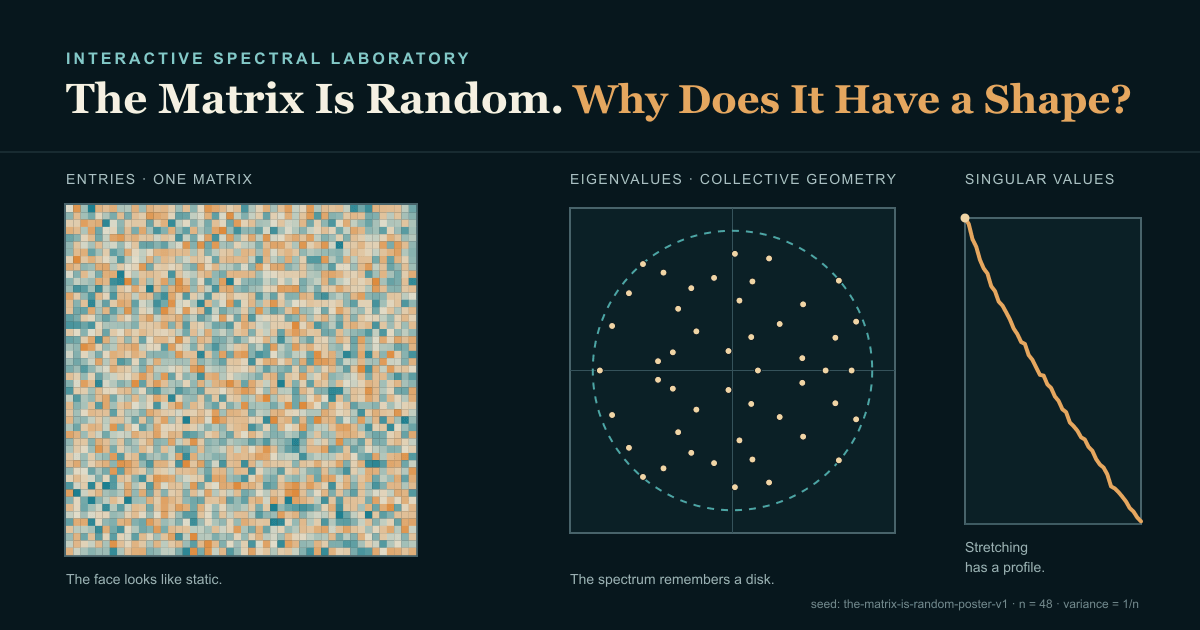
A square has already appeared before we have done any mathematics. Put $n^2$ random numbers in an $n\times n$ grid, colour the negatives blue and the positives amber, and the eye begins negotiations with the noise. There is a diagonal. There is a cloud. There is perhaps a face in the cloud, if one has slept badly enough.

Then ask a different question of exactly the same numbers. Compute the eigenvalues of a nonsymmetric matrix and place their real and imaginary parts on a plane. A rough disk appears. Make the matrix symmetric and the disk collapses onto the real line, where an arch-shaped density rises. Construct a covariance matrix and a different ridge occupies a sharply bounded interval. Repeat the experiment and the wandering points settle into laws.

The entries were random. The shapes are not drawings hidden in the entries. They are collective consequences of probability, algebra, normalization and the particular question being asked.

The heatmap asks where the numbers sit. The spectrum asks how the transformation acts. The singular values ask how strongly it stretches. The ensemble asks what survives repetition. These are not four pictures of the same fact.

RANDOM MATRIX LABORATORYSpectral sky

Waiting to begin

Exit focus mode

INTERACTIVE MATHEMATICS · SEEDED EXPERIMENT

One random matrix. Six ways to ask what shape it has.

The heatmap shows entries in one basis. The other lenses ask about collective statistics, invariant algebra, stretching, dynamics, and declared null models.

Save PNG Copy experiment URL Focus mode

Waiting to begin

0%

0%

The instrument will start when it nears the viewport.

PresetCircular cloud

Objectn = 64

Entriesgaussian · μ 0 · σ 1

Normalisationvariance-1/n

Seedtramlight-circle-1847

01Matrix02Spectrum03Singular04Direction05Structure06Ensemble

Preparing a deterministic matrix locally.

The article remains server-rendered while the browser loads a Worker and numerical routines near this viewport.

GUIDED EXPERIMENTS

Change one mathematical question

Undo last card

Let the circle gather Raise n and compare one spectrum with an ensemble.Hold the seed; change the scale Keep every draw fixed and remove the 1/√n normalisation.Make symmetry exact Watch complex eigenvalues collapse onto the real axis.Same spectrum, different face Compare A with QᵀAQ and audit the numerical discrepancy.Lift a signal from noise Increase a rank-one spike, then compare declared null statistics.Eigenvalues are not stretches Use the non-normal trap and compare ρ(A) with σ₁(A).Change microscopic noise Swap Gaussian entries for matched Rademacher entries.Persuade the eye Change only the colour encoding; the matrix stays fixed.Shuffle the same entries Destroy spatial arrangement while preserving the entry histogram.

Accessible data and numerical summary Waiting for the first result

The numerical tables will appear after the browser worker finishes the first seeded experiment.

Audio article

Uses the speech voice supplied by your browser or device.

1. A grid full of random numbers

The laboratory begins with a seed, not with Math.random(). A small deterministic pseudorandom generator turns the seed, matrix settings and sample number into a reproducible stream. Gaussian values are produced by a reproducible transform of that stream; uniform and Rademacher values use separate declared mappings. Rademacher sounds grander than it is: each entry is either $-1$ or $+1$ with equal probability before scaling.

For the default Circular cloud experiment,

Thus each displayed entry has variance $1/n$. The $1/\sqrt n$ is not cosmetic tidying. Without it, a typical spectral radius grows like $\sqrt n$ in this ensemble; with it, the interesting collective scale remains of order one as $n$ changes.

The Matrix microscope renders each entry as one nearest-neighbour rectangle. It does not blur adjacent cells into a smooth field. At a useful zoom it reveals the numerical value, row and column. The side profiles and histogram answer elementary questions—whether a row has drifted, whether values are centred, whether one column is unusually energetic—without claiming that a noisy local fluctuation is structure.

Three display transforms are deliberately separated:

• Raw shows the values used by the calculation.
• Standardized subtracts the displayed matrix mean and divides by its displayed standard deviation.
• Absolute value discards signs and therefore needs a sequential rather than diverging colour scale.

A threshold can suppress values below a chosen magnitude. That can be useful for inspection, but the surviving islands are produced jointly by data and threshold. Unless a control explicitly says otherwise, colour and threshold affect only the picture; the numerical engine continues to analyse the matrix stated in the status line.

2. Why the heatmap appears shapeless

Independent entries have no reason to arrange themselves into long smooth bands. A finite heatmap therefore resembles television static. That is not a failed visualization. It is an honest answer to one question: where did this particular draw place its individual values?

The eye is an eager compression algorithm. It joins nearby bright cells, mistakes a run for a stripe and assigns importance to a conspicuous corner. Change the colour limits, sort the rows by norm or interpolate between pixels and a bland field can become geological. The matrix has not confessed. The display has changed the terms of interrogation.

The rearrangement menu makes this visible:

• Independent entry shuffle preserves the bag of entry values but generally changes eigenvalues, singular vectors and every row relationship.
• Joint row-and-column permutation computes $PAP^T$. This is a similarity transformation, so a square matrix keeps its eigenvalues while its heatmap is rearranged.
• Orthogonal change of basis computes $Q^TAQ$. It also preserves eigenvalues, while spreading local-looking features across a new coordinate system.
• Order by row norm may produce a smooth envelope because the sorting rule explicitly asked for one. It is not a similarity transformation and need not preserve the spectrum.
• Spectral ordering sorts coordinates by the components of a largest-magnitude eigenvector for a symmetric matrix, or by the leading left singular vector for a nonsymmetric matrix, and then applies the same order to rows and columns as $PAP^T$. Its block-like appearance is evidence about that declared procedure before it is evidence about the world; the joint permutation, not the sorting criterion, is why the eigenvalues survive.

The Same spectrum, different face experiment places $A$ beside $Q^TAQ$. Their corresponding eigenvalues agree to a displayed numerical tolerance although the cell patterns can look unrelated. This is the cleanest warning in the room: appearance in one basis is not an algebraic invariant.

3. A matrix transforms space

An $n\times n$ matrix is not only an array. It defines a linear transformation

It stretches some directions, contracts others, mixes coordinates and can turn a vector into one pointing somewhere else. In two dimensions a unit circle becomes an ellipse. In $n$ dimensions a unit sphere becomes a high-dimensional ellipsoid that no laptop screen can display whole.

The Direction machine therefore labels itself as a projection. It chooses a declared two-dimensional plane, draws vectors in that plane, applies the full matrix, and projects the results back for display. This can reveal strong stretching, rotation or transient amplification in the selected plane. It cannot prove that every invisible direction behaves the same way.

Repeated application starts from $\mathbf x_0$ and calculates

When requested, each step is normalized so that direction remains visible after the magnitude would otherwise overflow or vanish. Growth, shrinkage, rotation, sign alternation and alignment are reported separately. The spectral radius helps describe long-run exponential behaviour, but for a non-normal matrix it need not describe the largest short-run excursion.

4. Eigenvalues: directions and rates that survive

An eigenpair satisfies

The direction $\mathbf v$ is returned to itself, scaled by $\lambda$. For a real symmetric matrix, eigenvalues and eigenvectors are real and an orthonormal eigenbasis exists. A general real matrix is less polite.

Consider the quarter-turn matrix

No non-zero real vector keeps its direction after a quarter-turn. Its eigenvalues are $+i$ and $-i$. Complex eigenvalues are therefore not imaginary decoration: a conjugate pair encodes a real invariant plane in which scaling and rotation occur together. The Spectral sky retains both components and plots $\lambda=a+ib$ at $(a,b)$. Discarding $b$ would turn a rotation into a false pair of zeros.

Because a real matrix has a real characteristic polynomial, non-real roots occur in conjugate pairs. The plot keeps equal geometric scale on its real and imaginary axes, includes zero lines and exposes each selected value as text: real part, imaginary part, magnitude and angle.

5. The circular law

For an $n\times n$ matrix with independent, mean-zero, variance-$1/n$ entries, the empirical eigenvalue distribution approaches the uniform distribution on the unit disk under broad conditions as $n$ grows. This is the circular law. The unit circle in the instrument is a large-$n$ reference, never a hard finite-sample fence.

The modern universality result by Tao, Vu and Krishnapur makes the striking point precise: after the stated centring and variance normalization, the limiting empirical spectral distribution does not depend on the full microscopic entry distribution under the theorem’s assumptions (Annals of Probability, 2010).

That is why the Universality test can switch among Gaussian, uniform and Rademacher entries after matching their first two moments. Their individual heatmaps remain recognizably different—Rademacher has only two raw values—yet their large-scale spectral clouds can become similar. The browser provides an illustration, not a proof. Finite dimensions, tail behaviour and local statistics still matter.

Click Accumulate once and the single cloud remains ragged. Add ten matrices and the disk becomes plausible. Add one hundred within the device budget and a stable density begins to appear. Nothing in that sequence turns a finite point cloud into an exact theorem; it shows how an ensemble statement becomes visible only through repetition.

6. Symmetry changes everything: the Wigner semicircle

Now impose $A=A^T$. The lower triangle is no longer independent of the upper triangle, and the spectral picture changes category. Every eigenvalue is real. The two-dimensional sky becomes a one-dimensional density.

For the normalization used by Wigner moonrise, off-diagonal entries have variance $1/n$. In the large-$n$ limit the density approaches

and zero outside $[-2,2]$. The curve is a semicircle in the density plot, not because the matrix heatmap contains an arch but because many correlated algebraic contributions settle into that limiting distribution. Wigner developed random-matrix models while studying statistical regularities in complicated nuclear resonance levels (Cambridge Philosophical Society, 1951); his 1955 matrix paper is part of that historical line (Annals of Mathematics).

The overlay again states assumptions and scale. Change to an incompatible normalization and the instrument rescales the theory correctly where the mapping is defined; otherwise it disables the curve rather than leaving a confident lie on the chart.

7. Covariance and the Marchenko–Pastur ridge

The Wishart ridge starts from a rectangular $n\times m$ data matrix $X$ with independent, mean-zero, variance-one entries and forms

$C$ is symmetric positive semidefinite, so its eigenvalues are real and non-negative. Let

In the high-dimensional limit, the continuous part of the Marchenko–Pastur distribution lives between

This law goes back to the 1967 paper by Marchenko and Pastur (Mathematics of the USSR-Sbornik). If $\gamma>1$, then $n>m$ and the rank of $C$ is at most $m$; at least $n-m$ eigenvalues are exactly zero in exact arithmetic. The instrument shows the zero mass rather than squeezing it into the continuous ridge.

This is the geometry behind a common difficulty in high-dimensional covariance estimation: when the number of variables is not small relative to the number of observations, sample covariance eigenvalues spread even under a featureless null model. A large-looking eigenvalue is not automatically a substantive principal component.

8. Eigenvalues and singular values answer different questions

Every real $m\times n$ matrix has a singular-value decomposition

where the diagonal entries of $\Sigma$ satisfy

The singular values are the square roots of the eigenvalues of $A^TA$. They measure how strongly the transformation stretches orthogonal input directions. They remain meaningful for rectangular matrices and do not become complex.

The Singular-value mountain plots the descending profile, cumulative squared energy and a documented numerical rank. Its tolerance is based on matrix size, machine precision and the largest singular value; the status line exposes it. A condition number

is reported as effectively infinite when the smallest relevant value falls beneath that tolerance. Near singularity, a long string of impressive digits would be theatre.

Drag the rank $k$ to form the truncated reconstruction

The microscope then displays the best rank-$k$ approximation in the Frobenius and spectral norms—the Eckart–Young result (Psychometrika, 1936)—with reconstruction error calculated from the retained decomposition. A random dense matrix usually compresses poorly. A planted low-rank signal may appear earlier, although noise can still dominate the raw heatmap.

For a normal matrix, singular values are the magnitudes of eigenvalues. For a non-normal matrix they can differ dramatically. That difference is not a bug; it is one of the main reasons to inspect both.

9. One matrix is an anecdote; an ensemble is a population

A matrix ensemble is a probability model for generating matrices. A statement about one realization and a statement about the ensemble have different logical subjects.

The laboratory’s accumulation is paused by default. Starting it advances through deterministic sample indices, never through frame-rate-dependent randomness. The seed and parameters determine sample zero, sample one and every later sample regardless of how quickly the browser draws them. Pausing, hiding the tab or changing a colour scale does not mutate the mathematical sequence.

At one sample, an edge fluctuation can look like an outlier. At ten, a bulk begins to form. At one hundred, a stable empirical distribution may become visible. The appropriate sample cap falls as $n$ rises because each eigendecomposition becomes more expensive. A large matrix and a large ensemble are competing uses of a finite computation budget.

The density field is therefore withheld until enough points exist. Before that, dots are more honest than a smooth contour that suggests more evidence than has been collected.

10. Normalization changes the picture

“Random matrix” is not a complete experimental specification. Mean, variance, symmetry, sparsity and normalization all alter the spectrum.

The instrument offers four explicit scales:

1. Unscaled variance leaves the selected entry variance independent of $n$; many spectral magnitudes then grow with dimension.
2. Dimension-scaled entries multiply the declared scale by $1/\sqrt n$, giving standard deviation $\sigma/\sqrt n$ and variance $\sigma^2/n$. The familiar variance-$1/n$ case is recovered at $\sigma=1$ and is the canonical scale for the circular and Wigner presets.
3. Frobenius normalization divides by $\lVert A\rVert_F$, forcing the total squared entry energy to one.
4. Spectral-radius normalization divides a square matrix by $\rho(A)=\max_i|\lambda_i|$ when that value is numerically usable.

The last two are data-dependent transformations. They make some comparisons convenient but change the ensemble and couple every entry through a global statistic. Theoretical overlays derived for independent variance-$1/n$ entries do not silently survive that operation.

A non-zero mean is equally consequential. Writing

exposes a rank-one mean component. A leading eigenvalue or singular value can separate from the noise bulk. “The entries are random” has not prevented a deterministic collective direction from being present.

11. Colour scales and sorting manufacture structure

A diverging colour map makes zero a perceptual centre and uses two distinguishable directions for sign. A sequential map is appropriate for magnitude, density or another one-sided quantity. Neither choice is innocent, but some choices match the quantity better than others.

Three common manufacturing operations deserve suspicion:

• Clipping at a robust quantile gives ordinary values more contrast but hides the full range.
• Thresholding creates islands by definition and changes discontinuously when the threshold crosses a value.
• Sorting converts a statistic into spatial order; a smooth band may simply be the graph of the sort key.

Change only the colour scale in the final reader experiment. The underlying matrix, eigenvalues, singular values and test statistics remain fixed. Notice how easily visual confidence moves while the mathematics does not.

12. Same spectrum, different face

If $Q$ is orthogonal, then

is the same linear transformation expressed in a rotated orthonormal basis. Indeed,

The eigenvalues agree. Individual entries need not. Local-looking structure in a heatmap can dissolve because locality belonged to the chosen coordinates, not to the abstract linear operator.

Singular values also survive an orthogonal change on both sides. Arbitrarily sorting rows alone, however, computes $PA$, not $PAP^T$; that generally changes eigenvalues. The interface names these operations separately because a vague “reorder” button would conceal the central distinction.

The room metaphor is useful only if returned to mathematics. A heatmap is the arrangement of furniture in one coordinate room. The spectrum asks about certain modes of motion through the building. Redrawing the coordinate axes can move every item on the floor plan without changing basis-invariant algebraic quantities.

13. Add a faint signal to noise

The Structure detector begins with a null matrix $X$ and adds a controlled alternative. Its simplest form is

For the symmetric rank-one experiment, $\mathbf v=\mathbf u$. Other alternatives plant a two-block mean, a diagonal band, Toeplitz-like correlation, sparse hubs, a repeated motif, a non-zero mean or unequal row variance.

The slider moves $\alpha$ continuously. At low strength the signal may be invisible in the heatmap. A singular statistic may nevertheless drift. At larger strength an outlier can detach from the spectral bulk. Finite-rank perturbations can have genuine spectral phase transitions; the precise threshold and outlier formula depend on the ensemble and perturbation model (Benaych-Georges and Nadakuditi, 2011).

The original Baik–Ben Arous–Péché transition concerns a particular spiked complex sample-covariance model (Annals of Probability, 2005). The instrument does not lazily label every separating dot “BBP”. Its Wigner spike, rectangular singular-value spike and Wishart spike are identified according to the model actually being calculated.

14. Unusual relative to what?

For the selected matrix, the detector calculates a restrained set of declared statistics: largest singular value, spectral radius, a leading real eigenvalue where applicable, inverse participation ratio for the selected eigenvector (compared with the same eigenvalue-magnitude rank in each null draw), row or column correlation, low-frequency power and contrasts matched to planted structures.

It then generates independent matrices from the selected null ensemble, applies the same statistic and reports an empirical percentile or standardized deviation. The language is intentionally conditional:

• Ordinary under this null model means the observed statistic sits in the common part of this finite null sample.
• Unusual under this null model means it lies in a tail of that comparison.
• Insufficient ensemble samples means there is not enough resolution for strong language.
• The result depends on the chosen null model is always true, even when a short status line omits repeating it.

This is not a universal pattern detector. A Gaussian dense null is inappropriate for a sparse degree-heterogeneous network; an IID null is inappropriate for time-correlated measurements; a covariance null may need estimated nuisance structure. A result becomes unusual only after the comparison class has been declared.

Testing seven metrics, trying six colour scales and reporting only the most exciting result creates a multiple-comparisons problem. Selection changes the false-discovery risk; the warning is statistical rather than moral (Benjamini and Hochberg, 1995). The detector keeps its declared metrics visible and refuses to combine them into one theatrical “signal found” badge.

15. Sparse galaxies and localized eigenvectors

Dense random-matrix laws rely on density and moment assumptions that can fail in sparse regimes. In Sparse galaxy, most potential edges are absent, the remaining values are centred and a few vertices may have unusually high degree.

Isolated vertices can create zero eigenvalues. Hubs can create outliers. An eigenvector may localize on a small set of coordinates rather than spread its weight broadly. One diagnostic is the inverse participation ratio

For a unit vector spread evenly across $n$ coordinates, the value is of order $1/n$; concentration on a few coordinates raises it. That number describes a computed vector in a chosen basis. It does not by itself identify a meaningful community or causal hub.

16. The non-normal trap

A matrix is normal when $A^TA=AA^T$ in the real case. Symmetric matrices are normal; many nonsymmetric matrices are not.

The Non-normal trap uses a nearly upper-triangular transformation with a small perturbation. Its eigenvalues may all lie comfortably inside the unit circle, suggesting eventual decay, while some vectors grow strongly for several iterations before decay wins. Non-orthogonal eigenvectors can cancel at one moment and reinforce at another.

For non-normal matrices, eigenvalues alone can be a poor guide to finite-time behaviour. Pseudospectra ask how the spectrum can move under small perturbations, equivalently examining the smallest singular value of $zI-A$ across the complex plane. Trefethen’s review gives the precise warning: spectra of far-from-normal operators may say little about norms of powers or matrix exponentials (SIAM Review).

This browser instrument deliberately does not compute a pseudospectrum: even a coarse complex-plane grid would require another singular-value decomposition at every grid point, while still being easy to overread as a precise boundary. Instead the repeated-direction view, the gap between $\rho(A)$ and $\sigma_1(A)$, and the definition through $\sigma_{\min}(zI-A)$ explain the non-normal warning without borrowing the stronger diagnostic name.

17. What the picture can—and cannot—prove

What the picture can—and cannot—prove

• A visually striking pattern is not automatically statistically significant.
• A single realization does not establish an ensemble law.
• Theoretical laws are asymptotic and depend on assumptions.
• Finite matrices depart from ideal limiting distributions.
• Colour, interpolation, thresholds and sorting can invent apparent structure.
• Random-looking data may contain planted structure.
• Structured-looking data may still arise by chance.
• A result is unusual only relative to a declared null model.
• Pseudorandom output is reproducible and algorithmic.
• Numerical decomposition has finite precision and stability limits.

The numerical warning beside a decomposition is part of the result. Standard numerical linear algebra treats accuracy and stability as properties to measure, not assume (Higham, 2002). Residuals such as

and

are checked against scale-aware tolerances where the corresponding vectors are available. A nearly defective matrix can have accurate-looking eigenvalues and ill-conditioned eigenvectors. No browser library repeals floating-point arithmetic.

18. Applications, with the simplifications left attached

Random-matrix theory is useful because high-dimensional noise has structure of its own. The toy ensembles here are reference models, not automatic portraits of real systems.

• Covariance estimation and PCA: Marchenko–Pastur behaviour helps explain why sample eigenvalues spread when variables and observations are comparable in number. Spiked models study when a low-rank population feature separates from this noise. Real data may be heavy-tailed, dependent, missing or heteroscedastic.
• Noisy scientific measurements: a null spectral bulk can provide a baseline for separating coherent low-rank variation from instrument or sampling noise. The scientific design must still supply the correct noise model.
• Wireless communication: large random channel matrices give tractable limits for multi-antenna capacity and signal-processing questions; Tulino and Verdú provide an authoritative treatment (Foundations and Trends in Communications and Information Theory). A browser IID matrix is not a complete radio channel.
• Neural networks: weight-matrix singular values influence how signals and gradients stretch through layers. Initialization studies use random-matrix ideas (Pennington, Schoenholz and Ganguli, 2017), but trained networks are structured, nonlinear and data-dependent.
• Dynamical systems: spectral radius, non-normality and pseudospectra help distinguish asymptotic stability from transient amplification.
• Graph spectra: adjacency and Laplacian eigenvalues can reflect degree structure, components and communities. Sparse graphs require models different from dense Wigner matrices.
• Financial covariance: random-matrix comparisons have been used to study noisy market correlation matrices (Plerou and colleagues, 1999). Markets are non-stationary, dependent and reflexive; a bulk comparison does not turn a historical covariance estimate into a safe trading rule.
• Nuclear energy levels: random matrices entered physics partly as statistical models for spectra too complicated to derive level by level. They model selected statistics of an ensemble, not the detailed nuclear Hamiltonian.
• Low-rank signal in high-dimensional noise: spectral separation provides both a practical method and a warning: below a model-dependent threshold, a real signal can remain entangled with the bulk.

The ramifications are epistemic as much as technical. Noise is not necessarily flat. High-dimensional null models can have sharp edges, preferred scales and predictable extreme behaviour. Seeing a large eigenvalue is therefore only the start of a question.

19. Experiments worth trying

The experiment cards inside the instrument change the required controls together and preserve a route back to the prior state.

1. Grow the circular cloud. Increase $n$ while retaining variance $1/n$, then accumulate samples. Watch the boundary become statistically clearer without becoming exact.
2. Hold the seed, change the scale. Switch among unscaled, variance-$1/n$, Frobenius and spectral-radius normalization. Notice which theoretical overlay remains justified.
3. Trade Gaussian for Rademacher. Keep the first two moments fixed. The heatmap changes microscopically; the large spectral cloud may change much less.
4. Make it symmetric. Watch complex conjugate pairs collapse to a real density and the semicircle reference replace the unit disk.
5. Change the face, keep the spectrum. Compare $A$ with $Q^TAQ$ and inspect the numerical agreement rather than trusting the heatmaps.
6. Raise a rank-one signal slowly. Find the region where the heatmap remains ambiguous while an extreme singular value begins to look unusual under the null.
7. Enter the non-normal trap. Compare eigenvalue magnitudes, singular values and the maximum norm reached under repeated application.
8. Shuffle the entries. Record which summaries survive a bag-of-values-preserving shuffle and which depended on row, column or spectral structure.
9. Persuade your own eye. Freeze everything except the colour scale, threshold and sorting rule.

Sources and further reading

• Terence Tao, Van Vu and Manjunath Krishnapur, “Random matrices: Universality of ESDs and the circular law”, The Annals of Probability 38(5), 2010.
• Eugene P. Wigner, “Characteristic Vectors of Bordered Matrices With Infinite Dimensions”, Annals of Mathematics 62(3), 1955.
• V. A. Marchenko and L. A. Pastur, “Distribution of Eigenvalues for Some Sets of Random Matrices”, Mathematics of the USSR-Sbornik 1(4), 1967.
• Jinho Baik, Gérard Ben Arous and Sandrine Péché, “Phase Transition of the Largest Eigenvalue for Nonnull Complex Sample Covariance Matrices”, The Annals of Probability 33(5), 2005.
• Florent Benaych-Georges and Raj Rao Nadakuditi, “The Eigenvalues and Eigenvectors of Finite, Low Rank Perturbations of Large Random Matrices”, Advances in Mathematics 227(1), 2011.
• Lloyd N. Trefethen, “Pseudospectra of Linear Operators”, SIAM Review 39(3), 1997.
• Carl Eckart and Gale Young, “The Approximation of One Matrix by Another of Lower Rank”, Psychometrika 1, 1936.
• Nicholas J. Higham, “Accuracy and Stability of Numerical Algorithms”, second edition, SIAM, 2002.
• Antonia M. Tulino and Sergio Verdú, “Random Matrix Theory and Wireless Communications”, Foundations and Trends in Communications and Information Theory 1(1), 2004.
• Vasiliki Plerou and colleagues, “Universal and Nonuniversal Properties of Cross Correlations in Financial Time Series”, Physical Review Letters 83, 1999.
• phase space, “I Tried Making Generative Art (p5js)”, used only as a seed for the spirit of generative experimentation. Its code, graphics, structure, wording and branding are not used here; the mathematical and numerical claims above come from the cited literature and stated calculations.

Randomness can be shapeless at the level of individual entries yet lawful at the level of collective behaviour. The surprise is not that noise can be made beautiful. It is that the shape depends on the question—and that a responsible picture tells us which question it answered.