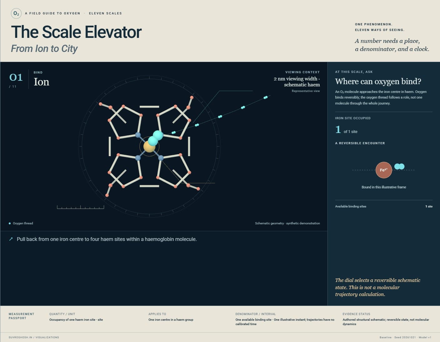
A field guide to oxygen · Eleven scales
The Scale ElevatorFrom Ion to City
A number needs a place,
a denominator, and a clock.
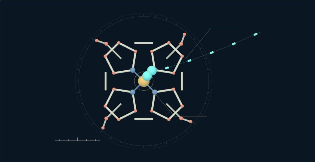
Ion
Pull back from one iron centre to four haem sites within a haemoglobin molecule.
passport
A declared synthetic reference at every floor.
Held constant: SaO₂ 98%; PaO₂ 100 mmHg; Hb 15 g/dL; cardiac output 5 L/min at the centre dial.
Baseline synthetic reference. The local dial changes only the active floor’s declared parameter.
Read the eleven-floor field guide
- 01 / 2 nm viewing width · schematic haem
Ion: Where can oxygen bind?
An O₂ molecule approaches the iron centre in haem. Oxygen binds reversibly; the oxygen thread follows a role, not one molecule through the whole journey. A local binding state cannot describe a person’s oxygen status.
Occupancy of one haem iron site · site · One available binding site · One illustrative instant; trajectories have no calibrated time. Authored structural schematic; reversible state, not molecular dynamics.
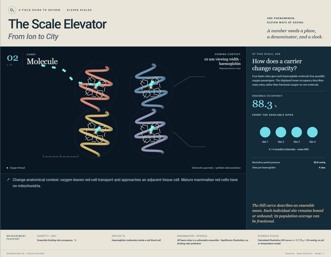
- 02 / 10 nm viewing width · haemoglobin
Molecule: How does a carrier change capacity?
Four haem sites give each haemoglobin molecule four possible oxygen passengers. The displayed mean occupancy describes many sites, rather than fractional oxygen on one molecule. A fraction means little until its denominator is known.
Ensemble binding-site occupancy · % · All haem sites in a schematic ensemble · Equilibrium illustration; no binding-rate prediction. Calculated illustrative Hill curve: n = 2.7, P₅₀ = 26 mmHg; no pH or temperature model.
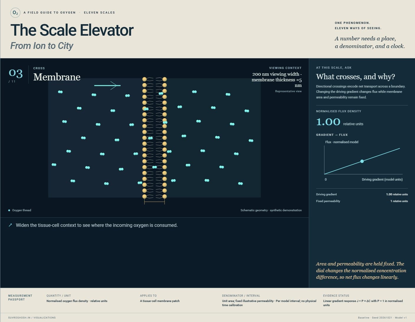
- 03 / 200 nm viewing width · membrane thickness ≈5 nm
Membrane: What crosses, and why?
Directional crossings encode net transport across a boundary. Changing the driving gradient changes flux while membrane area and permeability remain fixed. A concentration gradient drives transport; flux also depends on permeability and area.
Normalised oxygen flux density · relative units · Unit area; fixed illustrative permeability · Per model interval; no physical time calibration. Linear gradient response J = P × ΔC with P = 1 in normalised units.
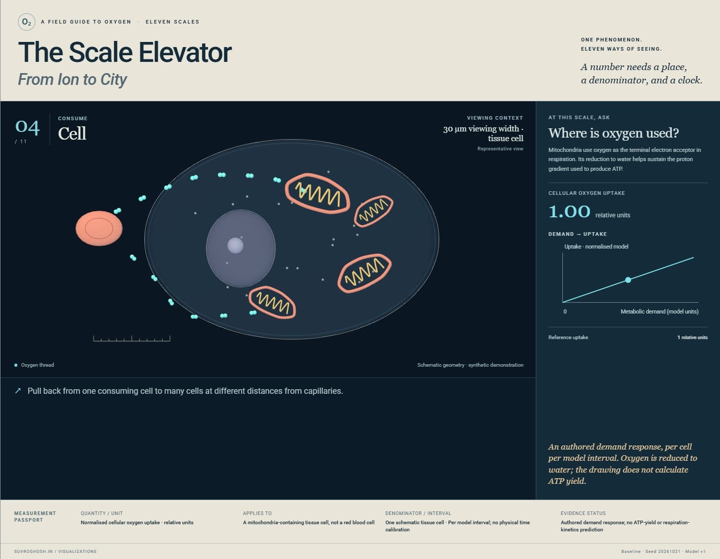
- 04 / 30 µm viewing width · tissue cell
Cell: Where is oxygen used?
Mitochondria use oxygen as the terminal electron acceptor in respiration. Its reduction to water helps sustain the proton gradient used to produce ATP. Oxygen is consumed in respiration; it does not turn directly into ATP.
Normalised cellular oxygen uptake · relative units · One schematic tissue cell · Per model interval; no physical time calibration. Authored demand response; no ATP-yield or respiration-kinetics prediction.
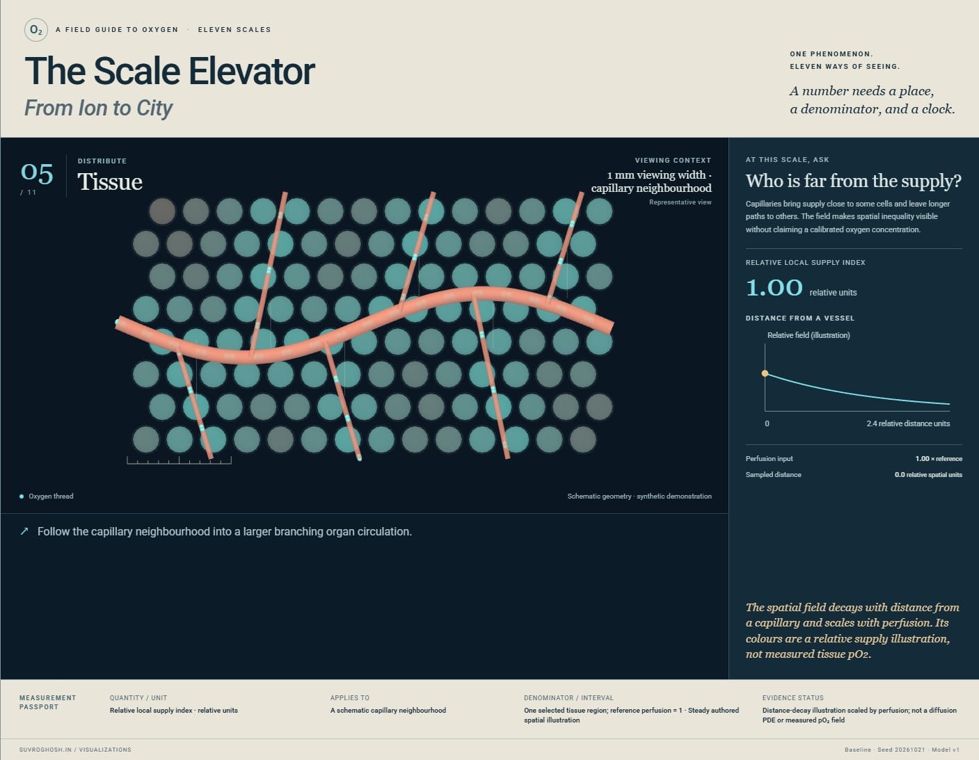
- 05 / 1 mm viewing width · capillary neighbourhood
Tissue: Who is far from the supply?
Capillaries bring supply close to some cells and leave longer paths to others. The field makes spatial inequality visible without claiming a calibrated oxygen concentration. A tissue-wide average can conceal local shortage.
Relative local supply index · relative units · One selected tissue region; reference perfusion = 1 · Steady authored spatial illustration. Distance-decay illustration scaled by perfusion; not a diffusion PDE or measured pO₂ field.
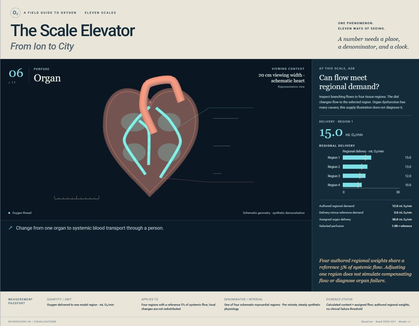
- 06 / 20 cm viewing width · schematic heart
Organ: Can flow meet regional demand?
Inspect branching flows to four tissue regions. The dial changes flow to the selected region. Organ dysfunction has many causes; this supply illustration does not diagnose it. Regional flow and demand can differ even when whole-body totals look sufficient.
Oxygen delivered to one model region · mL O₂/min · One of four schematic myocardial regions · Per minute; steady synthetic physiology. Calculated content × assigned flow; authored regional weights, no clinical failure threshold.
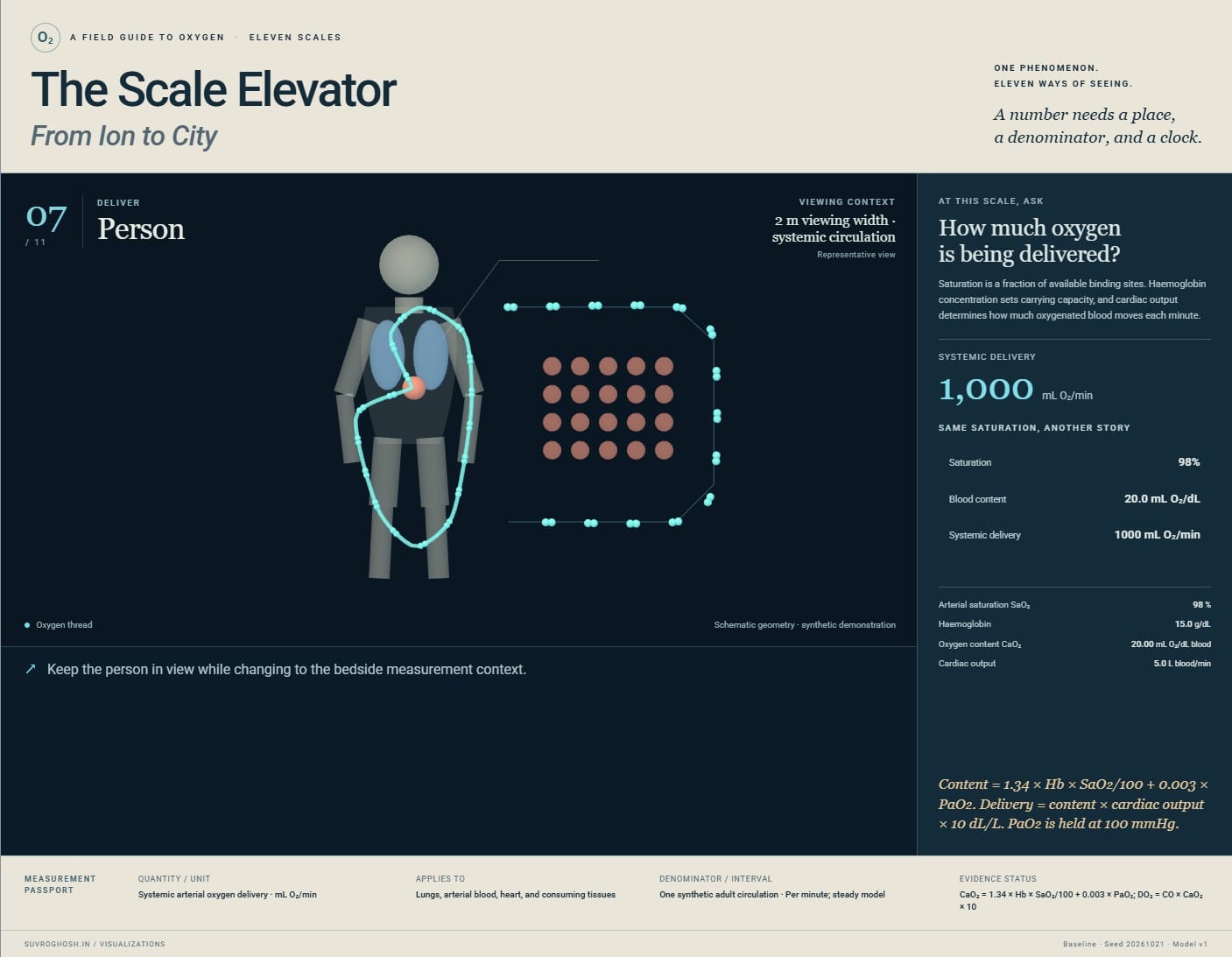
- 07 / 2 m viewing width · systemic circulation
Person: How much oxygen is being delivered?
Saturation is a fraction of available binding sites. Haemoglobin concentration sets carrying capacity, and cardiac output determines how much oxygenated blood moves each minute. The same saturation can coexist with different oxygen content and delivery.
Systemic arterial oxygen delivery · mL O₂/min · One synthetic adult circulation · Per minute; steady model. CaO₂ = 1.34 × Hb × SaO₂/100 + 0.003 × PaO₂; DO₂ = CO × CaO₂ × 10.
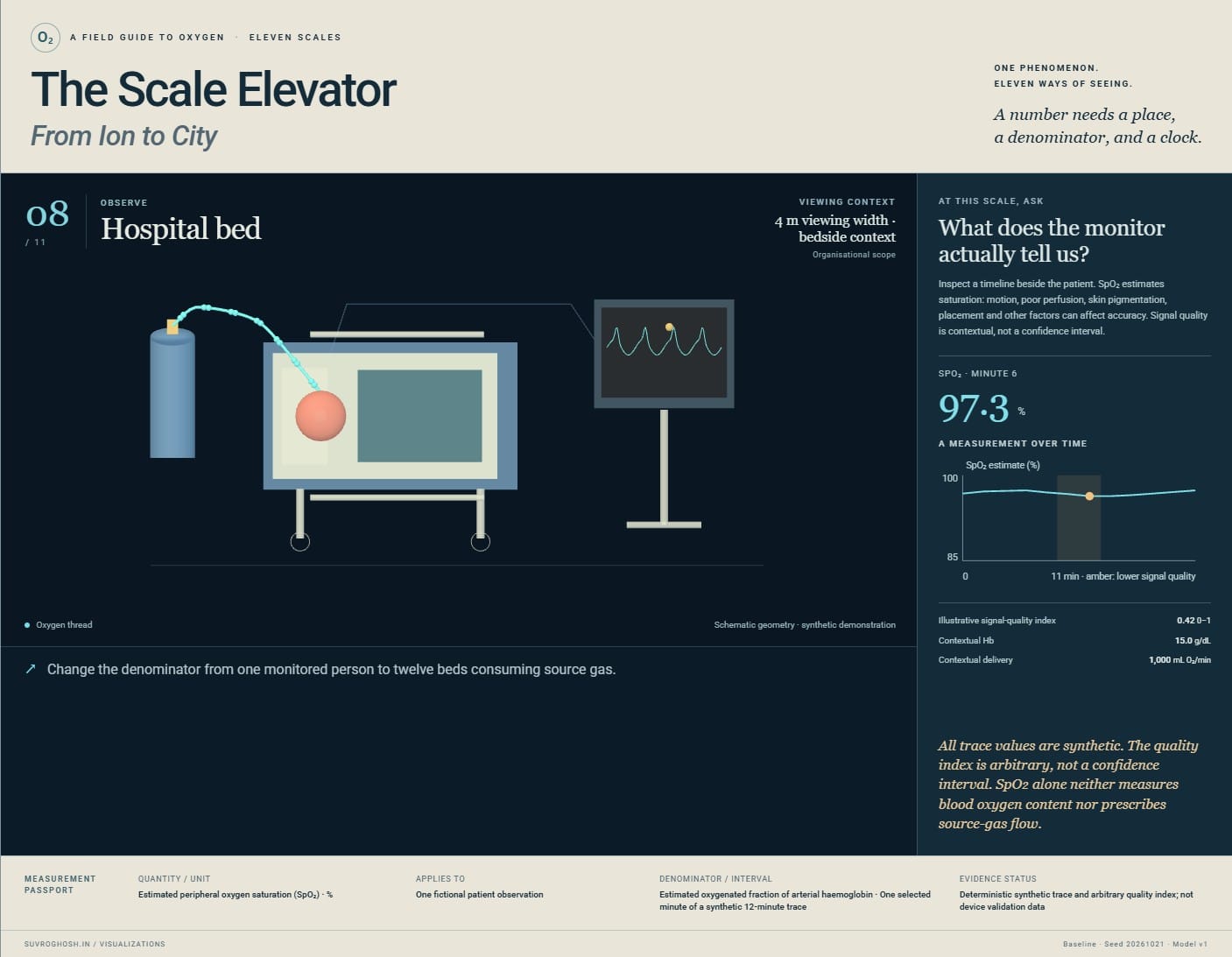
- 08 / 4 m viewing width · bedside context
Hospital bed: What does the monitor actually tell us?
Inspect a timeline beside the patient. SpO₂ estimates saturation: motion, poor perfusion, skin pigmentation, placement and other factors can affect accuracy. Signal quality is contextual, not a confidence interval. A monitor percentage is one observation, with uncertainty and clinical context.
Estimated peripheral oxygen saturation (SpO₂) · % · Estimated oxygenated fraction of arterial haemoglobin · One selected minute of a synthetic 12-minute trace. Deterministic synthetic trace and arbitrary quality index; not device validation data.
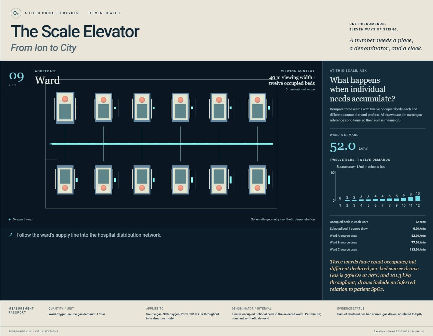
- 09 / 40 m viewing width · twelve occupied beds
Ward: What happens when individual needs accumulate?
Compare three wards with twelve occupied beds each and different source-demand profiles. All draws use the same gas-reference conditions so their sum is meaningful. Equal occupancy does not imply equal oxygen-service demand.
Ward oxygen-source gas demand · L/min · Twelve occupied fictional beds in the selected ward · Per minute; constant synthetic demand. Sum of declared per-bed source-gas draws; unrelated to SpO₂.
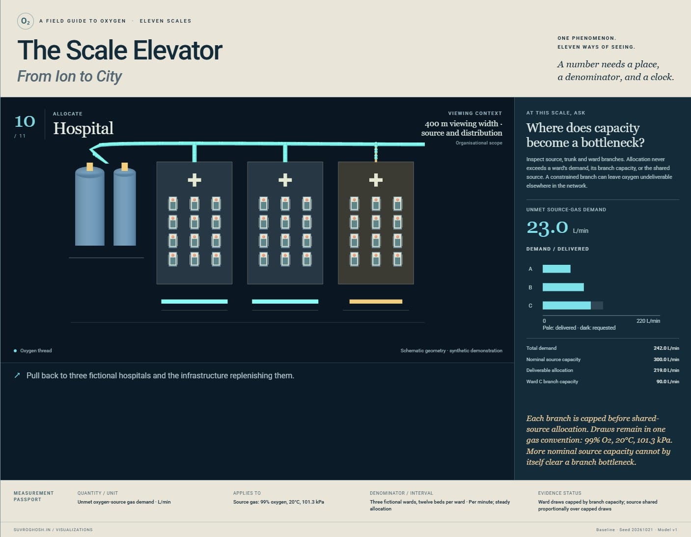
- 10 / 400 m viewing width · source and distribution
Hospital: Where does capacity become a bottleneck?
Inspect source, trunk and ward branches. Allocation never exceeds a ward’s demand, its branch capacity, or the shared source. A constrained branch can leave oxygen undeliverable elsewhere in the network. Nominal source capacity can hide a constrained ward connection.
Unmet oxygen-source gas demand · L/min · Three fictional wards, twelve beds per ward · Per minute; steady allocation. Ward draws capped by branch capacity; source shared proportionally over capped draws.
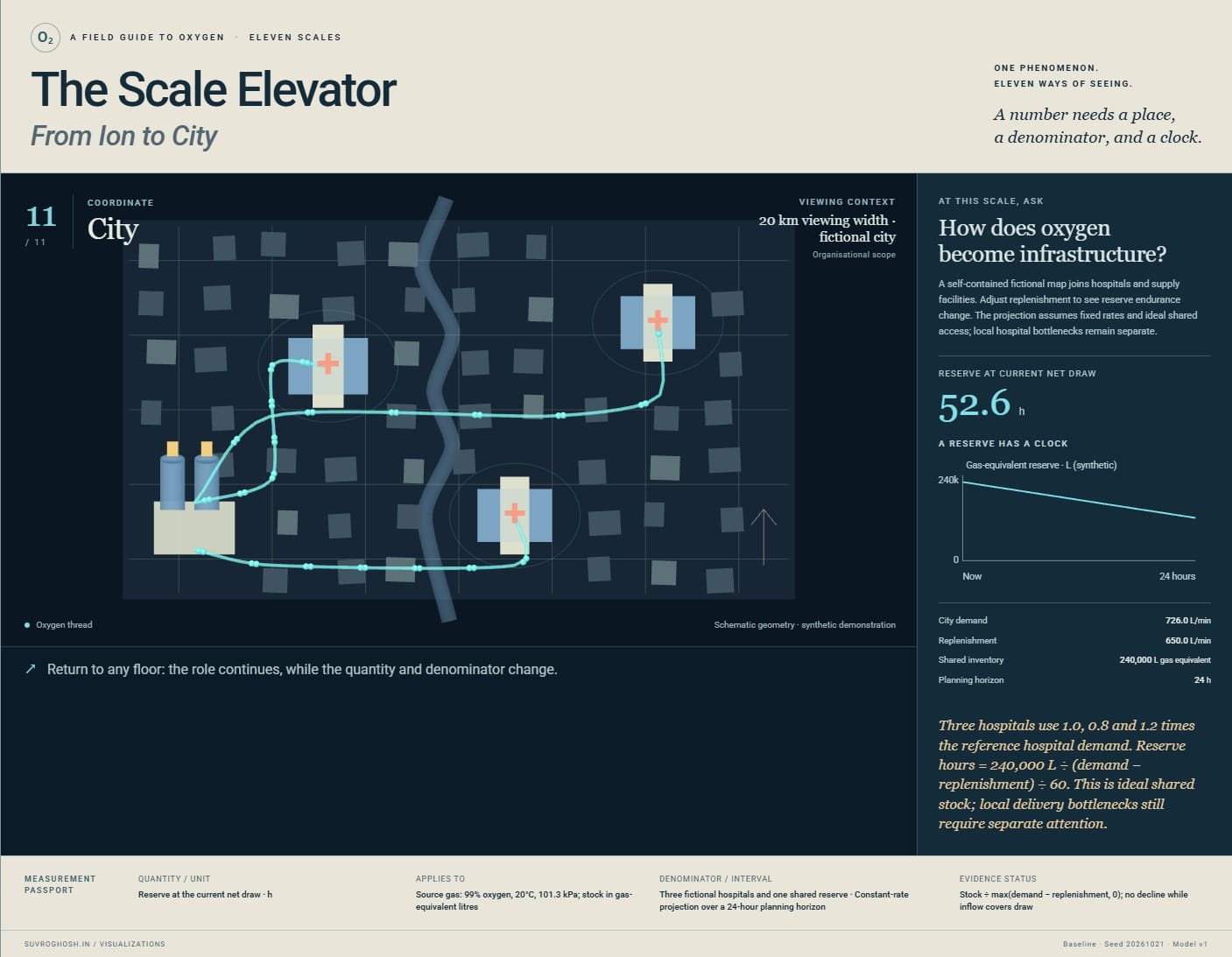
- 11 / 20 km viewing width · fictional city
City: How does oxygen become infrastructure?
A self-contained fictional map joins hospitals and supply facilities. Adjust replenishment to see reserve endurance change. The projection assumes fixed rates and ideal shared access; local hospital bottlenecks remain separate. Oxygen becomes a problem of geography, replenishment, resilience and time.
Reserve at the current net draw · h · Three fictional hospitals and one shared reserve · Constant-rate projection over a 24-hour planning horizon. Stock ÷ max(demand − replenishment, 0); no decline while inflow covers draw.
About this model, its units, and its limits
This is a synthetic educational exhibit. Geometry, molecular motion, local flux, uptake and tissue fields are schematic. The haemoglobin content and delivery examples use declared physiological equations; the ward and city examples use a separate source-gas accounting model.
A saturation percentage, an oxygen delivery rate, and a hospital gas flow are different quantities. The source network assumes 99% oxygen gas at 20°C and 101.3 kPa throughout. Source demand includes device gas use and is not a conversion from a person’s oxygen uptake. Inventory is expressed as gas-equivalent litres.
There are no real patient records, live capacity feeds, clinical predictions, or treatment thresholds. The iron-to-haemoglobin view is followed by an explicit handoff to an adjacent tissue cell. Physical extent changes into anatomical and organisational context as the journey expands.
The local dial applies to the currently interpreted floor. Scenarios hold their declared comparison variables constant. The article below gives the equations, assumptions, references, and distinctions in full.
Published · Updated
Uses the speech voice supplied by your browser or device.
What does an oxygen level belong to?
A person looks at a bedside monitor and sees a percentage. A ward manager looks at a gas supply and sees litres per minute. A delivery coordinator looks at a store and asks how long it will last. All three are looking after oxygen. Their numbers answer different questions.
The Scale Elevator begins at the iron centre of a haem group and ends above a fictional city. Between them lie a carrier protein, a membrane, a cell, tissue, an organ, a person, a hospital bed, a ward and a hospital. Each stop changes what we can see and what it makes sense to count.
The continuous journey is a visual argument: a quantity needs an object, a unit and a context. A beautiful number with its context removed can be more misleading than an untidy explanation with its assumptions attached.
Every clinical record and infrastructure scenario here is synthetic. The small-scale scenes are explanatory constructions. The exhibit joins several educational models; its camera does not turn them into one complete simulation of a living body.
Taking the lift
Move the scale slider, select a floor, or start the guided tour. Previous and Next make the same journey a step at a time. You can pause, reverse direction and revisit a view while keeping the selected comparison. The local control belongs to the current floor; its label explains what it changes.
Read the measurement passport alongside the picture. It names the quantity, unit, scope, time interval and denominator, and identifies synthetic, calculated or illustrative values. The physical viewing extent appears separately. A membrane’s thickness is not the width of the frame containing its diagram.
The views change continuously, but their measurements do not blend. Halfway between a cell and a tissue diagram, an intermediate camera position has no biological meaning of its own. Some handoffs reveal a larger structure; others deliberately change anatomy, measurement or organisation.
Eleven ways to ask about oxygen
01 · Ion: a place to bind
The first scene centres on iron within haem. The approaching object is molecular oxygen, O₂. Reversible attachment gives the opening a small, local question: is this site occupied? The surrounding ring supplies context for the metal centre.
The paths are authored trajectories, not molecular dynamics. Their purpose is to distinguish approach, binding and release. The RCSB PDB-101 account of haemoglobin describes the relationship between iron-containing haem groups and oxygen transport.
02 · Molecule: a denominator appears
The view opens to schematic haemoglobin and its four haem sites. Counting occupied sites becomes useful only beside the number available. A single molecule has discrete occupancy; an ensemble permits a fraction.
Inspect the illustrative binding response as the control changes. It compresses a complex interaction into a bounded teaching relationship. The protein geometry and particle paths are drawn for explanation rather than reconstructed from crystallographic coordinates.
03 · Membrane: a boundary becomes the subject
A cross-section replaces the protein portrait. The useful vocabulary becomes sides, gradients and crossings. The display’s normalised transport response makes the declared driving difference visible without claiming a calibrated membrane permeability.
This is also an anatomical handoff. Haemoglobin carries oxygen inside red blood cells; the journey now turns towards a tissue cell. A healthy mature human red blood cell lacks mitochondria. The exhibit does not give the carrier cell the consuming tissue cell’s machinery. Research on abnormal mitochondrial retention in sickle red blood cells illustrates why this anatomical distinction matters.
04 · Cell: arrival is followed by use
Compartments replace trajectories as the organising picture. Oxygen reaches mitochondria in a schematic tissue cell and participates in respiration. The uptake display uses a declared illustrative demand relationship.
At this handoff the persistent oxygen motif changes meaning. We are following a role, not an indestructible molecule. Oxygen is reduced to water in the respiratory chain; it does not turn directly into ATP. RCSB’s explanation of cytochrome c oxidase places oxygen consumption within the machinery that supports cellular energy conversion.
05 · Tissue: the average loses its address
Capillaries and neighbouring cells spread across a field. Select a region near a vessel and another farther away. The picture can no longer be read as one cell’s uptake: location and distance now matter.
The oxygen-related field is an authored spatial model, not a solved diffusion experiment. The four inspection points use relative distances, while the passport separates the selected supply index from the perfusion input. Which regions disappear when we replace the entire patch with one average? A reassuring centre can coexist with a poorly supplied edge inside the illustration.
06 · Organ: supply meets unequal demand
A schematic heart introduces branching flows and regional supply. Lowering the perfusion control changes the model’s delivery illustration. Four fixed synthetic demand references remain unchanged as delivery varies. Inspecting a region reveals its delivery, declared demand and the difference; a fixed chart scale keeps the comparisons visible.
This view illustrates transport stress. It does not diagnose organ failure. A coloured region is an output of a simplified relationship, while real dysfunction involves interacting processes that this picture does not represent. The change of visual vocabulary makes a limited claim easier to inspect.
07 · Person: a percentage needs a carrier
The whole-person view links lungs, circulation and consuming tissues. It separates saturation from arterial oxygen content and systemic delivery. The calculation uses haemoglobin concentration, saturation and partial pressure, then multiplies content by blood flow with the necessary unit conversion.
The educational approximation is:
Here is in g/dL, saturation in percent, partial pressure in mmHg and flow in L/min. Content is expressed in mL O₂/dL blood and delivery in mL O₂/min. The factor ten converts litres of blood to decilitres. The oxygen-transport physiology reference gives this content approximation. It is not a model of compensatory circulation.
08 · Hospital bed: a measurement acquires a history
The person becomes a bedside scene with a synthetic monitoring timeline. Inspect a point and read its time and signal-quality context. The trace belongs to an observation process; its vertical movement is not a direct film of oxygen molecules.
SpO₂ estimates blood oxygen saturation. Circulation, skin pigmentation, temperature and other factors can affect accuracy, as the FDA explains. The exhibit’s signal-quality labels are authored examples, not an algorithm for certifying a reading. The contextual haemoglobin and flow values come from separate declared inputs.
09 · Ward: addition needs compatible units
A ward plan replaces the bedside timeline. Each bed contributes a synthetic oxygen-service demand. Selecting beds makes their contribution to the total visible.
These are compatible source-gas flow rates under one stated reference condition and purity. They can be added. Saturation percentages cannot be added to produce gas demand. Two occupied beds may place very different demands on an oxygen service, even before a ward’s distribution limits enter the picture.
10 · Hospital: a total needs a route
Sources, storage, distribution and wards form a network. Inspect a constrained connection and compare available supply with deliverable flow. A large nominal source can coexist with unmet demand at a branch.
The allocation rule is explicit and bounded. It explains a bottleneck without claiming to engineer a medical pipeline. The WHO specifications for facility oxygen systems treat sources, storage and distribution as distinct parts of a functioning service. This exhibit’s network is fictional.
11 · City: a reserve needs a clock
The final view becomes a map because geography and connections now organise the question. Three fictional facilities share a supply story. Demand and replenishment act over a stated horizon; inventory is an amount, while supply and use are rates.
Explore reduced replenishment or higher demand, then return to the bedside. The journey back is useful: a hospital’s reserve is consequential to a person, but it does not describe that person’s saturation. Likewise, a good bedside reading cannot certify a city’s resilience.
Three comparisons worth carrying upstairs
Same saturation, different haemoglobin. Hold the declared saturation, partial pressure and flow constant while reducing haemoglobin concentration. The calculation changes oxygen content and delivery. It deliberately leaves compensatory responses outside the model.
Same content, different blood flow. Hold the blood’s calculated content constant and reduce flow. Delivery changes because the amount passing through each minute changes. A still image of blood composition cannot answer a question about transport per minute.
Same beds, different service demand. Keep occupancy fixed and change the synthetic source-demand profile. The ward totals change; the hospital allocation and city balance then expose consequences under their own assumptions. The comparison never derives a gas prescription from an SpO₂ trace.
A selected comparison may leave a molecular mechanism unchanged. That is a useful result: an upstream drawing should not twitch merely because a downstream planning assumption changed.
Keeping the units attached
The physiological equations and the infrastructure ledger meet through an explicit educational handoff. They are not connected by a concealed conversion from blood oxygen delivery into a flowmeter setting. Source gas, inspired gas and oxygen consumed by tissue have different boundaries.
Infrastructure volumes here refer to synthetic gas-equivalent litres at 20 °C and 101.3 kPa with fixed 99% source purity. Stored inventory uses the same convention. It does not describe a vessel’s geometric volume or a changing pressure inside a cylinder. The network omits pressure dynamics, leaks, maintenance, clinical prioritisation and real procurement.
The molecular geometry, membrane response, cellular uptake, tissue field and organ comparison are simplified teaching devices. Patient traces and demand records are synthetic. These boundaries belong beside the exhibit because smooth motion can make a chain of illustrations feel more physically complete than it is.
A visual grammar that changes with the question
The exhibit draws on the editorial ambitions of Information Graphics, Knowledge Is Beautiful and Alberto Cairo’s The Functional Art: make relationships legible, organise attention, and choose an encoding for the question a reader needs to answer.
Trajectories become crossings, compartments, fields, flows, timelines, networks and maps. A recurring oxygen colour carries the thread while labels preserve the changing meaning. Three.js supplies the stage; HTML and SVG keep explanations and measurements readable around it. The scale rail is an index of contexts rather than a ruler of eleven equally spaced powers of ten.
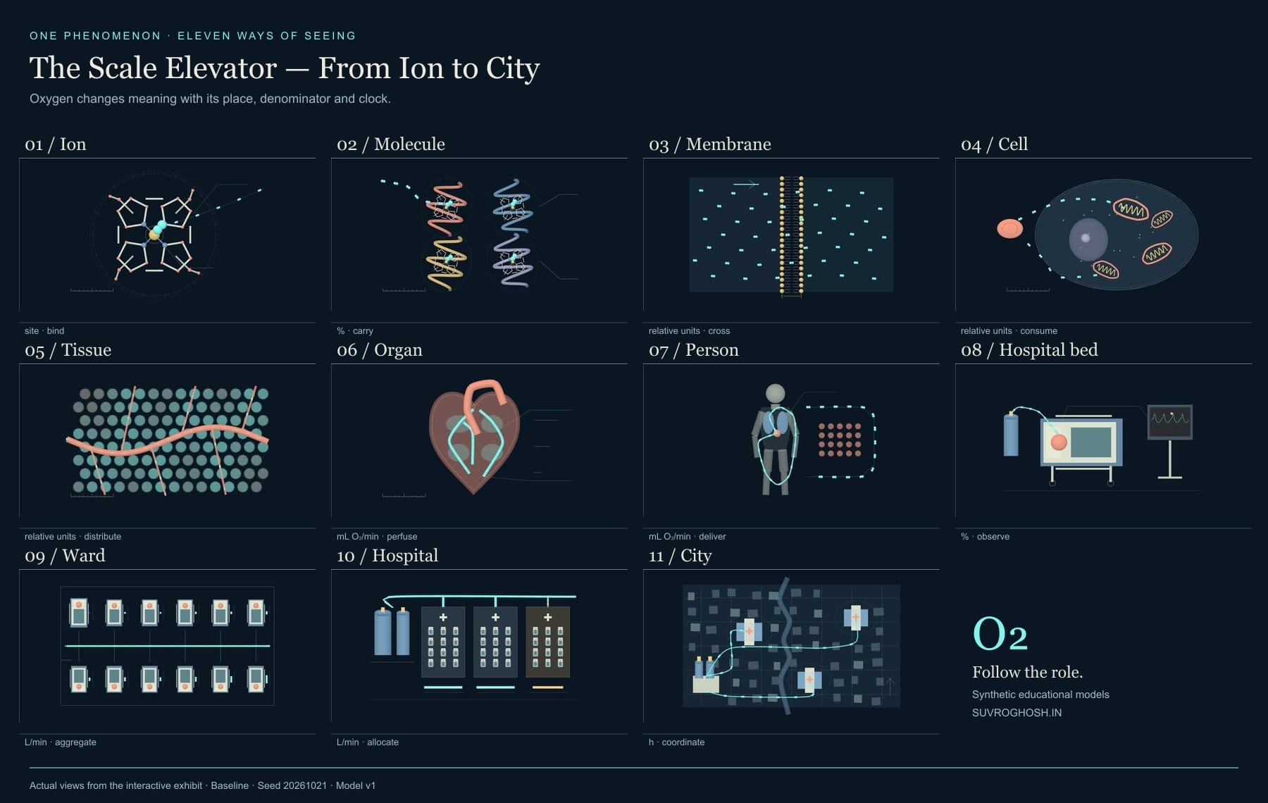
The recording travels through the same scenes as the interactive view. The stills preserve its individual stops. Either route should leave a useful habit behind: before interpreting a quantity, ask what it belongs to.
Quick reference and FAQ
Oxygen connects an iron binding site with a city's supply network, but the useful measurement changes along the way. Explore eleven scales and compare saturation, carrying capacity, blood flow, device demand and available supply without treating them as interchangeable.
Key Terms
- Semantic zoom
- Haem
- Haemoglobin
- Partial pressure
- Saturation
- Oxygen content
- Oxygen delivery
- Flux
- Aggregation
- Capacity
- Inventory
Frequently asked questions
Does one oxygen molecule travel through the entire exhibit?
No. The visual thread follows oxygen's role. Oxygen is consumed during cellular respiration, and later floors change anatomical context or organisational scope.
Does the ion floor show an oxygen ion?
It shows the iron centre in a haem group, where molecular oxygen, O₂, binds reversibly. The title describes the binding site's scale.
Can equal saturation mean different oxygen delivery?
Yes. In the declared educational calculation, arterial oxygen content also depends on haemoglobin concentration and partial pressure; delivery then depends on blood flow. The comparison holds other inputs constant.
Are the people, hospitals and city real?
All clinical traces, beds, wards, facilities and map locations are synthetic. The exhibit is an educational collection of models and authored illustrations.
Can I explore without animation or WebGL?
Yes. Reduced motion starts paused with manual floor controls. Still views, an ordered floor ledger and the article remain readable when WebGL or JavaScript is unavailable.
Word Cloud
Related reading
Selected by shared topics and section, with closer publication dates breaking ties.