The Static-Equilibrium Illusion: Life Refuses to Hold Still

What temperature, hormones, feedback loops, and predator–prey models reveal about dynamic balance

A bedside monitor draws a line from left to right. We want the trace to be orderly, yet the most reassuring pattern is not flat: it rises, falls and rises again. Life persists by moving—pushing matter and energy through cells, correcting disturbances, anticipating demands and sometimes generating rhythms of its own.

This essay takes its conceptual cue from Alan Garfinkel’s Newton Abraham Lecture and Xiong and Garfinkel’s question, “Are physiological oscillations physiological?”. The numerical claims below come from the linked clinical sources, experiments, datasets and reviews; the interactive curves identify when they are measurements, derived conversions or teaching models.

Audio article

Uses the speech voice supplied by your browser or device.

1. The flat-line opening

A flat line can mean that electrical activity has ceased. It can also mean a detached lead, a failed sensor, an averaging interval that erased fast variation, or a chart scaled too coarsely to show it. Flatness is therefore neither a general definition of health nor even, by itself, a diagnosis. It is an observation whose meaning depends on what was measured and how.

The same problem appears in less dramatic forms. A heart that never changes its interval is not the ordinary ideal. Breathing accelerates during exertion. Blood pressure responds to posture and sleep. Hormone secretion arrives in pulses. Core temperature tends to descend and rise across the day. The living question is not, “Did the number move?” but “Did it move in a viable way, at the right time, and recover or adapt when conditions changed?”

Biological stability is usually an activity, not a stillness.

2. One number lies by omission

“37°C” is useful shorthand, but it leaves out measurement site, time of day, age, recent activity and the person’s own pattern. In a study of young men of differing chronotype, the daily core-temperature excursion was approximately 1.1–1.3°C, with the minimum near 05:00 (Baehr and colleagues). That is a peak-to-trough excursion. Some disciplines call half that range an amplitude, so an unqualified “one-degree amplitude” is needlessly ambiguous. Nor is this study a universal constant for every body.

A blood-pressure reading is similarly conditional on cuff, posture, rest, medication and circadian phase. The common nocturnal “dip” is usually discussed as a percentage of daytime pressure, not as one invented number of millimetres of mercury; not everyone exhibits the typical pattern. Glucose means something different before a meal, after one and during illness. A single cortisol sample cannot reveal the faster pulses riding on its daily trend.

The four salivary cortisol values in the explorer—13.4 at waking, 20.4 thirty minutes later, 6.0 before lunch and 1.5 nmol/L at bedtime—need an especially careful label. They are model-estimated points for the “Normative” latent profile reported by Dmitrieva and colleagues, using 1,101 adults and 2,894 valid sampling days (study DOI). They are not raw sample means, serum reference values or a universal healthy curve, and four daily points cannot resolve ultradian secretion. Their horizontal positions are illustrative: the study’s collection moments were tied to waking, pre-lunch and bedtime, not fixed universal clock times.

One number is not false. It lies by omission when we forget its clock, context and method.

3. Homeostasis was never frozen matter

It would be historically wrong to blame Walter Cannon for equating physiology with literal thermodynamic equilibrium. His account of homeostasis allowed regulated variation. As Billman’s historical review emphasises, “steady states” in organisms are flexible and bounded, maintained by coordinated responses rather than perfect constancy.

The mistake is not homeostasis. The mistake is freezing homeostasis into one number. Several related ideas are easily collapsed into that static caricature:

Concept	What it means here
Thermodynamic equilibrium	No net macroscopic currents and no energy-driven organisation. A living organism as a whole is not in this condition.
Nonequilibrium steady state	Summary properties may remain statistically stable while matter and energy continue to flow. Modern nonequilibrium biological physics studies how such driven organisation persists.
Homeostasis	Regulation within viable bounds, potentially using several feedback loops, feedforward control, rhythms and context-dependent targets.
Allostasis	Predictive or adaptive adjustment—often glossed as “stability through change”. It is useful, but not a universally accepted replacement for homeostasis.
Stable fixed point	After a small perturbation, the system returns towards one dynamical state.
Stable limit cycle	After a small perturbation, the system returns towards a periodic orbit rather than one point.
Oscillation	The broader appearance of repeated change. It may be forced, transient, damped, noisy or self-sustained; a wavy trace alone does not prove a limit cycle.

“Homeodynamics” is a helpful emphasis: what remains viable is often maintained through change. It does not abolish homeostasis. It reminds us to ask about trajectories, timescales and mechanisms as well as ranges.

The distinctions also stop one scale from impersonating another. Thermodynamics describes constraints on physical processes; a fixed point or limit cycle describes the geometry of a particular mathematical system; homeostasis and allostasis organise physiological explanations. A body can maintain a nonequilibrium steady state while one subsystem approaches a fixed point and another follows a daily rhythm. “Dynamic” is not an alternative substance from which life is made. It is a demand that we specify what changes, what remains bounded and at which observational scale.

4. Open the time microscope

The explorer begins with three windows. At about twenty seconds, a representative 72-beat-per-minute heartbeat, a 15-breath-per-minute respiratory rhythm and a normalised pressure wave near 0.1 Hz occupy different facets because their units are not interchangeable. The heart and breathing rates have separate authoritative resting ranges; neither stylised trace is a diagnostic recording.

The arithmetic is simple but worth exposing. Seventy-two beats per minute converts to one beat every 0.833 seconds; it sits within the adult resting range of 60–100 beats per minute described by the US National Heart, Lung, and Blood Institute. Fifteen breaths per minute gives a four-second cycle, within the adult resting range of 12–20 reported by MedlinePlus. Those derived periods do not turn the illustrations into ECG or airflow data. The slower pressure trace is displayed only as a normalised oscillation near a ten-second period because the magnitude and even the contribution of proposed mechanisms vary (Julien, 2006).

At two hours, the view shifts to slower coordination. Lang and colleagues sampled ten healthy participants every minute for one to two hours and found regular basal glucose–insulin cycles in five of ten, around a representative 13-minute period, with glucose leading insulin by about two minutes (1979 experiment). The explorer’s smooth paired traces are a reconstruction of that summary, not a participant’s raw data. A 90-minute cortisol ripple represents a model setting at the upper edge of the 60–90-minute ultradian range described in Endocrine Reviews; it is not a row of measured samples.

Across twenty-four hours, temperature, normalised blood pressure and the sparse cortisol profile expose the cost of sampling without phase. An optional overlay rescales each signal to its own range. It is an “orchestra” of shapes, never a shared physiological y-axis.

An evidence-labelled time microscope

Living stability has a shape in time

Change the window, disturb a feedback loop, then intervene in a coupled ecosystem. The same instrument keeps measurements, reported ranges, mathematical models and disputed inferences visibly distinct.

Pause all motion

Fixed pointreturn towards one state

Limit cyclereturn towards one periodic orbit

Oscillationa pattern; mechanism still to be established

01

Time microscope · representative human rhythms

Open the shutter: seconds, hours, a day

Every row keeps its own unit and vertical scale. The shared horizontal axis is time—not an invitation to compare raw heights.

Representative rhythms, not medical reference values. Ranges, measured summaries, conversions and generated teaching curves remain labelled separately.

About 20 secondsAbout 2 hoursOne day

Show normalized orchestra

Drawn mark · Model-derived illustration

Numerical support · Derived conversion

Numerical support · Authoritative range

Heartbeat

Generated pulse shape; only its illustrative period is source-supported.

The generated trace uses 72 beats/min; the separately sourced adult resting range is 60–100 beats/min.

NHLBI — How the Heart Beats

Drawn mark · Model-derived illustration

Numerical support · Derived conversion

Numerical support · Authoritative range

Breathing

Generated sinusoid; only its illustrative cycle length is source-supported.

The generated trace uses 15 breaths/min; the separately sourced adult resting range is 12–20 breaths/min.

MedlinePlus — Normal adult breathing rate

Drawn mark · Model-derived illustration

Numerical support · Measured summary

Mayer pressure wave

Generated normalized sinusoid at the cited approximate frequency.

Frequency near 0.1 Hz is represented; amplitude is normalized because magnitude varies.

Julien (2006), Cardiovascular Research

Human-rhythm source drawer and exact display settings

Every displayed setting, evidence class, population and boundary.

Signal	Displayed setting	Evidence	Population / conditions	Source and limitation
Heartbeat	72 beats/min; 0.833 seconds/beat beats/min and seconds/beat	Derived conversionAuthoritative range	Adults at rest Illustrative 72 beats/min within the separately stated 60–100 beats/min range.	NHLBI — How the Heart Beats Donald & Lakatta (2023) — coupled cardiac pacemaker clocks The trace is an illustrative pulse rhythm, not a diagnostic ECG. Cardiac pacemaking couples membrane-voltage and intracellular calcium-clock mechanisms.
Breathing	15 breaths/min; 4 seconds/cycle breaths/min and seconds/cycle	Derived conversionAuthoritative range	Healthy adults at rest Illustrative 15 breaths/min within the separately stated 12–20 breaths/min range.	MedlinePlus — Normal adult breathing rate Fogarty et al. (2018) — respiratory rhythm generation and modulation Breathing is generated by central neural patterning and modulated by chemoreflex feedback. Rate varies with posture, activity, illness, medication and measurement conditions.
Mayer pressure wave	about 0.1 Hz; about 10 seconds normalized amplitude	Measured summary	Varies A normalized sinusoid represents the approximate frequency only.	Julien (2006), Cardiovascular Research Amplitude is deliberately normalized because magnitude and mechanism vary. A smooth teaching curve is not a blood-pressure recording.
Fast glucose–insulin oscillation	illustrative 13-minute cycle; glucose leads insulin by about 2 minutes within-signal normalized level	Measured summary	Ten healthy participants sampled every minute for one to two hours Regular basal cycles were reported in five of ten participants.	Lang et al. (1979), New England Journal of Medicine The smooth paired curves are stylized, not raw participant measurements. Values are normalized within each signal and must not be read as concentrations.
Cortisol ultradian activity	about 60–90 minutes; 90 minutes illustrated normalized modeled level	Measured summary	Varies A 90-minute ripple is used at the upper end of a reviewed 60–90-minute band.	Oster et al. (2017), Endocrine Reviews The ripple is model-derived, not a row of measured samples. Pulse timing and magnitude vary between people and across the day.
LH pulse timing as a GnRH surrogate	commonly 1–2 hours in early follicular phase; roughly 4 hours in luteal phase pulse interval	Authoritative range	Menstruating humans; timing depends on cycle phase LH is generally measured as a surrogate for hypothalamic GnRH pulses.	Endotext — The Normal Menstrual Cycle and the Control of Ovulation Cycle phase, age and sex matter. Estradiol feedback becomes positive near ovulation, so the ovarian cycle is not purely negative feedback.
Core temperature	24 hours; about 1.1 °C peak-to-trough excursion illustrated °C	Measured summary	Young men grouped by chronotype The study reported about 1.1–1.3 °C peak-to-trough depending on chronotype; nadir near 05:00.	Baehr et al. (2000), Journal of Sleep Research This is a representative curve, not a universal human constant. “Amplitude” can mean half the peak-to-trough range; this article uses the unambiguous full excursion.
Daily blood pressure	24 hours; sleep region illustrated at 85% % of daytime level	Measured summary	Varies Daytime is normalized to 100%; sleep is drawn inside the common 10–20% dipping range.	Huart et al. (2023), Hypertension review Not everyone exhibits normal nocturnal dipping. The display intentionally does not invent systolic or diastolic mmHg values.
Daily salivary cortisol	four summary moments across one day nmol/L	Model-derived illustration	Growth-mixture model of 2,894 valid days from 1,101 adults Model-estimated normative-profile points: waking 13.4; +30 minutes 20.4; pre-lunch 6.0; bedtime 1.5 nmol/L.	Dmitrieva et al. (2013), Psychoneuroendocrinology Four modeled class-profile points cannot resolve ultradian pulses. These salivary values are not serum reference values or individual trajectories. The study used event-relative collection moments, so their clock positions in the explorer are illustrative.

02

Feedback lab · generic dimensionless teaching model

How a brake becomes a metronome

Hold loop steepness fixed, then add delay. The same negative sign can restore, ring, or destabilize a fixed point depending on timing and sensitivity.

MODEL — not a patient model and not a claim about every physiological rhythm. The fixed-step solver changes only the teaching equation shown below.

Monotonic return τ = 0.00Damped ringing τ = 1.10Sustained oscillation τ = 1.40

Feedback steepness, n

4.0

Delay, τ

1.10

Perturbation

+0.60

Play Reset

Trace cursor · t = 15.75

current x(t) 1.160 delayed x(t−τ) 0.945

Time trace

Return after a +0.60 perturbation

Verified: successive peak-to-peak ranges shrink.

x(t)x(t−τ)unperturbed operating state

Memory view

Delay embedding

Delay embedding, not a two-variable phase portrait. When τ = 0, current and delayed values coincide on the diagonal.

Teaching equation

Production sees the past; loss acts now

dx/dt = a / [1 + (x(t−τ)/K)ⁿ] − bx

Production

falls as the delayed value rises

Removal

acts on the current value

Memory

τ shifts what the brake can “see”

Compact loop

A sign is not a tempo

production+x− after τproduction

• Instantaneous first-order negative feedback usually returns monotonically.
• Lag or inertia can produce overshoot and damped ringing.
• Sustained oscillation needs enough loop sensitivity together with sufficient phase lag, supplied here by delay; the nonlinearity shapes and bounds the cycle.

Feedback sources, verified presets and numerical boundary

Sources

• Xiong & Garfinkel — Are physiological oscillations physiological?
• Mackey & Glass — Oscillation and chaos in physiological control systems

Numerically checked presets

Preset	n	τ	Verification
Monotonic return	4	0.00	Verified: no equilibrium crossing; direct return.
Damped ringing	4	1.10	Verified: successive peak-to-peak ranges shrink.
Sustained oscillation	4	1.40	Verified: bounded late-cycle range persists after transients.

With a = 2, b = K = 1 and n = 4, the linearized first transition is τ ≈ 1.2092. The solver uses fixed-step RK4 method-of-steps at dt = 0.01 and equilibrium history.

Damped ringing preset selected.

03

Ecosystem lab · model, measurement, contested causal story

Intervene in a toy world; then face the field

Three panels use three different kinds of warrant. Their labels are part of the result.

Model

Shark Meets Tuna

Dimensionless teaching model—not a fit to shark or tuna field data.

Initial sharks

20

Initial tuna

40

Intervention time

5.0

Replay speed0.5×1×2×

Play Reset

Shared cursor · t = 14.40

sharks 16.91tuna 41.14

Prediction checkpoint

After removing ten sharks, what happens?

Sharks stay lower Exactly the old path Sharks may later overshoot

Remove 10 sharks

Synchronized trace

Populations through dimensionless time

tunasharksuninterrupted baseline

State-space view

Phase portrait

Coexistence: S* = β/q = 15; T* = δ/p = 13.33. The closed curves are neutrally stable—not an attracting biological limit cycle.

Tuna to sharks positive effectSharks to tuna negative effectPhase lag emerges from coupled changes; no explicit delay

Model equations, assumptions, exact values and teaching sources

Equations

dT/dt = βT − qSTdS/dt = −δS + pST

RK4 with dt = 0.01; β = 0.6, q = 0.04, δ = 0.4, p = 0.03. Deterministic and dimensionless.

Assumptions

• Homogeneous mixing
• Exponential tuna growth without sharks
• Exponential shark decline without tuna
• Encounters proportional to ST
• Fixed conversion efficiency
• No carrying capacity
• No age or spatial structure
• No seasons
• No alternative prey
• No fishing
• No stochasticity

• Teaching Dynamics to Biology Undergraduates
• Shark Meets Tuna lesson
• Insulin–glucose delay lesson

Selected exact model values; dimensionless.

Time	Baseline sharks	Baseline tuna	Intervention sharks	Intervention tuna
0.00	20.0000	40.0000	20.0000	40.0000
5.00	16.3793	2.2077	6.3793	2.2077
10.00	3.9918	8.5649	2.9182	21.5745
15.00	26.7322	35.0743	40.1777	5.0925
20.00	14.3542	2.1957	7.2817	1.9422
25.00	3.8082	10.2079	2.7096	17.8226
30.00	33.1466	27.6539	43.6331	7.7719

Measured field data

Kluane control grids and reported treatment effects

Snowshoe hares, food availability and a predator guild in Yukon—not a simple lynx–hare pair.

Local CC0 subset

Spring control-grid composite, Efford ML

Measured summaries with supplied 95% confidence limits. Connecting segments are visual guides, not continuous monitoring. This later archive composite is not a transcription of the 1995 paper figure, which used spring grid-level CAPTURE jackknife estimates.

Reported aggregate ratio

Control

1× reference

Ratios compare treatment density with control density at the same time.

Reference condition; not a treatment-effect estimate.

Reported aggregate ratio

Mammalian-predator exclosure

about 2×

Average reported across peak and decline phases; raptors could still enter.

No confidence interval reported for this aggregate ratio.

Reported aggregate ratio

Food addition

about 3×

Average reported across peak and decline phases.

No confidence interval reported for this aggregate ratio.

Reported aggregate ratio

Food + exclosure

about 11×

More-than-additive average; the paper reports a late-decline maximum near 36×.

No confidence interval reported for this aggregate ratio.

What the paper reported: exclosure roughly doubled density, food produced roughly a threefold effect, and their combination averaged about elevenfold and reached about thirty-sixfold late in the decline. Predator abundance lagged hares by roughly one to two years. Food plus exclosure delayed the decline; it did not eliminate it.

Field-data table, transformation, sources and limitations

Dryad workbook 3, Hares sheet, spring rows selected from rows 26–41.

Occasion	Decimal year	Hares/ha	Lower 95% CL	Upper 95% CL
Spring87	1987.25	0.17779166666666668	0.10613333333333333	0.3648
Spring88	1988.25	0.5216666666666667	0.40345	0.8588
Spring89	1989.25	0.93125	0.6936166666666667	1.1717499999999998
Spring90	1990.25	1.51375	1.2285	1.8733833333333334
Spring91	1991.25	1.01875	0.715	1.0776666666666666
Spring92	1992.25	0.2945833333333333	0.2117	0.44628333333333337
Spring93	1993.25	0.09166666666666667	0.05	0.175
Spring94	1994.25	0.06541666666666666	0.03303333333333333	0.14091666666666666

Transformation: Selected rows Spring87 through Fall94 and columns A, B, C, D and G; serialized without changing values. The component filters the eight spring rows for the 1987–1994 display window. Display labels round only at render time. Spreadsheet helper columns E and F were not used as confidence bounds. The local file preserves all 16 spring and autumn rows; this view selects the 8 spring rows. Bounds were copied, not recalculated.

Sources

• Dryad dataset 10.5061/dryad.684s1
• Krebs et al. 1995 experiment
• Later Kluane synthesis associated with the archive
• Higher-dimensional interpretation

Limits

• The experiment concerned hares, a predator guild and food availability—not a simple lynx–hare pair.
• Raptors could enter the mammalian-predator exclosures.
• Hares could cross treatment boundaries.
• Costly exclosure and food-plus-exclosure treatments were not fully replicated.
• Predation, food, movement, weather and other factors remained entangled.
• Density and survival effects did not necessarily combine in the same way.

Disputed inference

Sharks, rays and scallops: audit the arrows

A tidy causal diagram can outrun its evidence.

Proposed in 2007

Large sharks ↓ · cownose rays ↑ · scallops ↓

Myers et al. proposed that declines in large coastal sharks released rays and contributed to a bay-scallop collapse.

Challenged in 2016

Timing, diet, space and demography questioned

Grubbs et al. argued that the correspondence and mechanisms were insufficient or equivocal. That critique concerns this claimed cascade—not whether sharks can ever participate in trophic cascades.

A plausible causal chain—even a beautiful one—is not the same thing as decisive field evidence.

Ecosystem model ready. Choose a prediction before removing sharks.

The source drawers and exact-value tables matter as much as the motion. Heart pacemaking depends on coupled membrane-voltage and calcium-clock mechanisms. Central respiratory pattern generation is modulated by chemoreflex and other inputs. Light, sleep, meals and activity can force or entrain other rhythms. Luteinising-hormone pulses, often around every one to two hours in the early follicular phase and roughly every four hours in the luteal phase, are an imperfect surrogate for hypothalamic GnRH; phase, age and sex matter, and ovarian feedback becomes positive near ovulation (Endotext). “Negative feedback did it” is not a universal explanation.

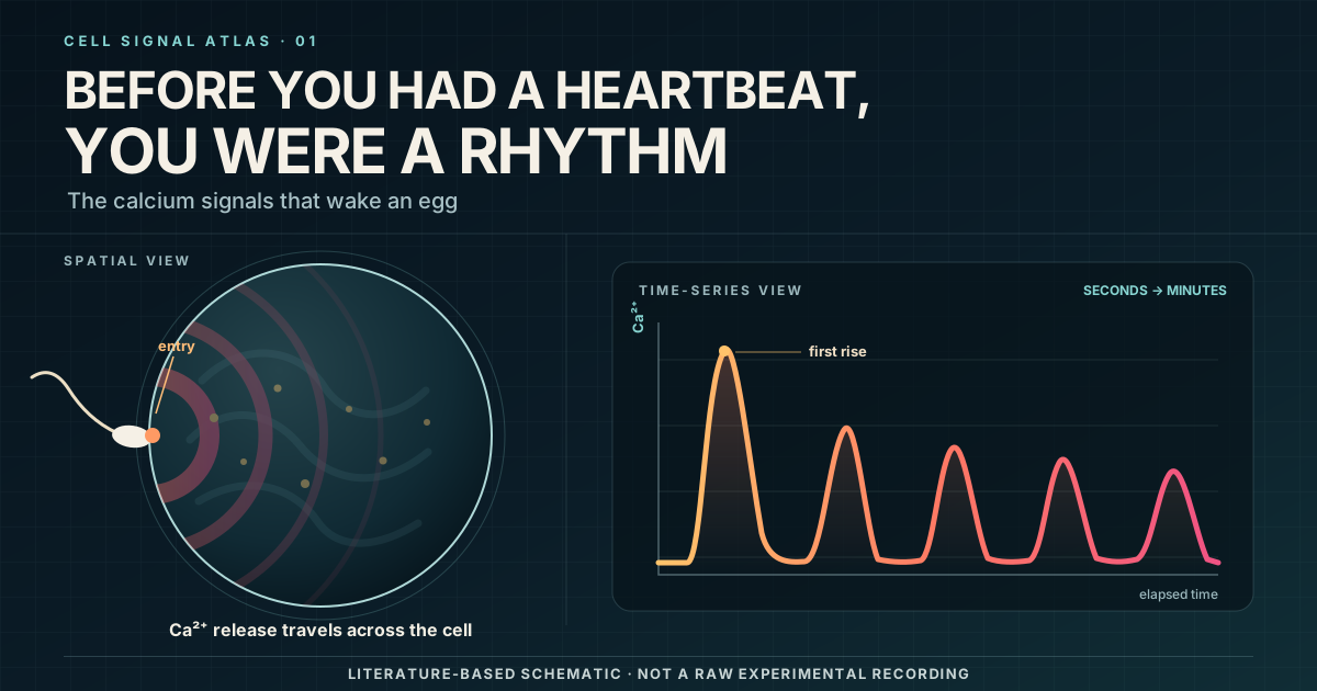
The companion essay Before You Had a Heartbeat, You Were a Rhythm follows another temporary biological clock: calcium waves and pulses that activate an egg.

5. How a brake becomes a metronome

The feedback lab isolates one mechanism. Its dimensionless equation makes production fall as the delayed state, x(t − τ), rises, while removal increases with the current state, x(t). It is a generic teaching model, not a patient model and not a claim about every physiological oscillator.

With instantaneous first-order negative feedback, a disturbance usually decays monotonically towards a stable fixed point: the brake responds to where the system is now. Introduce lag or inertia and the response may arrive after the variable has crossed its operating state. The correction then overshoots; a later correction overshoots in the other direction. With modest lag, those swings damp away.

Delay alone is not a magic oscillation switch. Sustained oscillation requires enough loop sensitivity together with sufficient phase lag—supplied here by delay; the nonlinearity shapes and bounds the resulting cycle. The lab’s “sustained” preset has been numerically checked to remain bounded and to keep cycling after its initial transient; it demonstrates one mathematical regime, not a healthy target. The classic delay analysis of blood-cell regulation by Mackey and Glass helped make this mechanism biologically legible.

The delay embedding plots x(t) against x(t − τ). It is not an ordinary two-variable phase portrait: both axes belong to the same variable at different times. By contrast, the unperturbed operating state is a fixed point. Increasing delay supplies phase lag; steepness changes loop sensitivity. Together they can move the fixed point through a stability threshold even though the feedback sign remains negative.

This is why the controls change one ingredient at a time. A larger perturbation tests the response without, by itself, changing the underlying rule. The Hill coefficient changes how abruptly production falls around its scale value. The delay changes which past state drives production now. “Damped” and “sustained” therefore describe the computed long-run behaviour of a specified parameter set; they are not decorative labels attached to traces that merely look wavy for a few seconds. Pause, scrub and inspect the exact values and the conclusion remains available without motion.

Other oscillators work differently: pacemaker ion channels, fast activation coupled to slow inhibition, interacting cells, molecular clocks, and external forcing by light, meals, activity or seasons. A brake can become a metronome. It does not follow that every metronome is a delayed brake.

6. From physiology to an ecological toy world

Garfinkel’s “Shark Meets Tuna” lesson moves the question from one delayed variable to two coupled populations. Tuna increase sharks through feeding; sharks decrease tuna through predation. In the ideal Lotka–Volterra equations, tuna grow exponentially without sharks, sharks decline exponentially without tuna, and encounters occur in proportion to the product of the two populations. The classroom context is described in Teaching Dynamics to Biology Undergraduates and the open Shark Meets Tuna lesson.

Remove ten sharks and the first effect looks obvious: fewer sharks. But more tuna then support shark growth; because the variables move out of phase, the later shark trajectory may rise above the uninterrupted baseline in this particular preset. The explorer forks the calculation at the intervention, preserves the dashed baseline and lets the reader compare both histories. It does not conceal the delayed consequence behind an animation.

The model uses a fourth-order Runge–Kutta integrator, but numerical care does not make its assumptions realistic. It has homogeneous mixing, fixed encounter and conversion rates, no carrying capacity, age structure, space, seasons, alternative prey, fishing or randomness. Its dimensionless preset is not fitted to shark or tuna observations. Adult sharks and tuna are not a canonical measured pair; their real relationships depend on species, sizes, locations and food-web context.

Most importantly, ideal two-species Lotka–Volterra dynamics form a neutrally stable family of closed orbits. Nearby trajectories do not converge on one attracting biological limit cycle. Its phase lag comes from coupled population change, not the explicit delay parameter used in the physiology lab.

For the displayed coefficients, the coexistence point is 15 sharks and about 13.33 tuna in dimensionless units. Starting exactly there would produce a flat mathematical solution; starting elsewhere selects one of the closed orbits. That flat solution is not “healthier” than the orbit, and neither is evidence about an actual fishery. It simply shows that the visual pattern follows from initial conditions as well as equations. The intervention matters because it changes the state mid-course: it places the same equations on a different orbit rather than commanding the system to return to its old calendar of peaks.

7. Then confront the toy with field evidence

An elegant model earns attention by clarifying a possibility. Field evidence must then face weather, movement, multiple species and limited replication. The eight-year Kluane experiment in Yukon manipulated winter food and access by mammalian predators while following snowshoe hares through a population cycle (Krebs and colleagues, 1995).

The headline effects were large: predator exclosure roughly doubled hare density on average, food addition produced roughly a threefold effect, and food plus exclosure produced a more-than-additive effect of about elevenfold on average—reaching approximately thirty-sixfold late in the decline. Predator numbers lagged hare abundance by roughly one to two years. Even the combined treatment delayed rather than eliminated the decline. These findings argue against a one-lever story.

The explorer deliberately does not draw four invented continuous treatment curves. Its local data table preserves the spring rows of the control-grid composite in the public Dryad archive, including 95% confidence limits. That later archive composite uses an Efford maximum-likelihood estimator; it is not an exact reproduction of the grid-level spring estimates made with CAPTURE’s jackknife procedure for the 1995 paper’s figure. The treatment ratios are shown separately as reported aggregate summaries, not manufactured by multiplying the control series.

The distinction is not clerical fuss. A smoothed line, an estimator, an experimental treatment and a published verbal summary answer different questions. The dataset provides valuable observations, but not a ready-made four-treatment time series with comparable uncertainty for every point.

Kluane is also not a simple lynx–hare pair. Hares faced a predator guild as well as food limitation. Raptors could enter exclosures; hares could cross their boundaries; the costly exclosure treatments were not fully replicated. Predation, food, movement, weather and other forces remained entangled, and density and survival effects did not necessarily combine in the same way. A higher-dimensional analysis by Stenseth and colleagues is a reminder that even a famous cycle may require more state variables than its iconic two-species sketch.

8. An elegant story is not field proof

The temptation to turn a plausible chain into a settled cascade reappears at sea. Myers and colleagues proposed that declines in large coastal sharks released cownose rays from predation, allowing ray predation to help collapse scallop populations. The story has the appealing sequence of a textbook model: sharks down, rays up, scallops down.

Grubbs and colleagues challenged the temporal correspondence, diet evidence, spatial assumptions and ray-demography argument. Their critique does not prove that sharks never cause trophic cascades. It changes the strength of this particular inference.

A plausible causal chain—even a beautiful one—is not the same thing as decisive field evidence.

That is why the explorer labels this panel DISPUTED INFERENCE, beside but not equivalent to MODEL and MEASURED FIELD DATA. Mathematical possibility, controlled observation and retrospective causal interpretation are different kinds of knowledge.

9. Guardrails

Restoring time to biology does not make every rhythm healthy. Arrhythmias, seizures, tremor and endocrine dysregulation are dynamic too. Some healthy regulation approaches a stable fixed point; some variables cycle; some are episodic or noisy. Regularity can be pathological, and variability can be either adaptive or dangerous depending on mechanism and scale.

Nor should a reader diagnose from these illustrative traces. Human rhythms vary with age, sex, menstrual phase, chronotype, sleep and light exposure, meals, activity and posture, illness, medication, assay method and measurement site. A resting range is not a forecast for exercise; a group summary is not an individual’s prescription; a normalised curve is not a concentration.

Snapshot measurements and reference ranges remain clinically indispensable. They make rapid decisions possible, support comparisons and reveal dangerous departures. The purpose here is narrower: add the missing time coordinate, then ask whether phase, history, rate of change or coupling alters the meaning of the snapshot.

Sometimes the next useful measurement is another sample after a defined interval. Sometimes it is a continuous record, a challenge test, a comparison with sleep or meals, or simply a repeat made with the same method. Sometimes timing contributes little and an urgent threshold is exactly what matters. The dynamic view is not a ritual demand for more data; it is a way to choose observations that match the process and the decision.

The same discipline applies to models. A model can reveal counterintuitive consequences without predicting a particular patient or ecosystem. A field result can constrain a model without proving every link in a narrative. Good visualisation keeps those epistemic labels attached.

10. Closing

The static-equilibrium illusion survives because a point is easy to print, remember and compare. But an organism is not a printed point. It is an open, driven history of flows and corrections, nested clocks and changing demands. Health is not motion for motion’s sake. It is the capacity to keep moving within, and sometimes deliberately shift, the conditions that make continued life possible.

The line matters. So do its scale, phase, provenance, neighbours and destination.

The body does not defend a number. It defends a viable dance.