The Predator–Prey Loom

By Suvro Ghosh · Published 7 November 2026 · Updated 7 November 2026

More food can support more prey. That gives predators more to eat, but their population takes time to respond. By the time predator numbers have risen, prey may already be declining.

This visualisation lets you follow that sequence. Add food, reduce the predator population, or change how effectively predators hunt. Watch what happens to both populations—and whether their earlier pattern returns.

Why do predator numbers often peak after prey numbers—and how can increasing the food available to prey produce larger population swings?

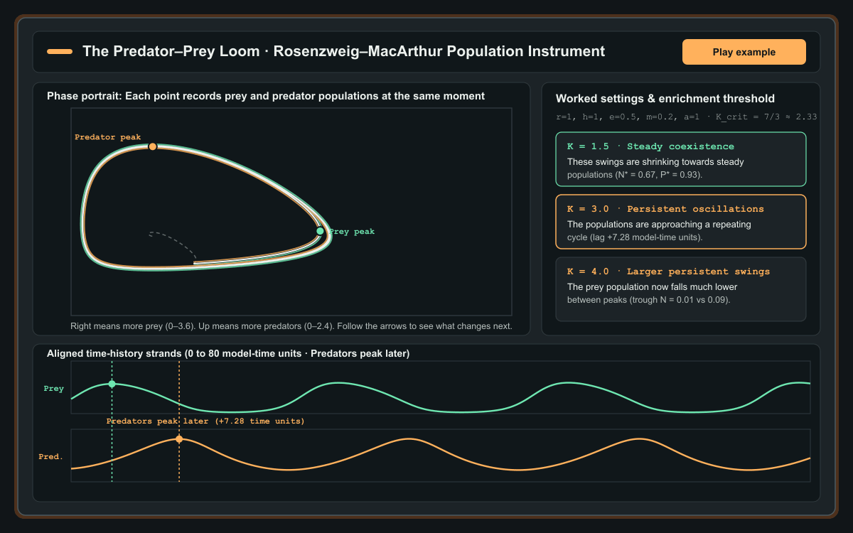
Using the Rosenzweig–MacArthur predator–prey model (illustrative population densities N for prey and P for predators over model-time units), the phase portrait records both populations at the same moment (“Right means more prey. Up means more predators. Follow the arrows to see what changes next.”), while the two aligned time-history tracks below show that predators peak later than prey. For the starting configuration (r = 1, h = 1, e = 0.5, m = 0.2, a = 1), the coexistence equilibrium loses stability at K = 7/3 ≈ 2.33: oscillations settle towards steady coexistence at K = 1.5, form a persistent repeating cycle at K = 3.0, and produce larger swings with lower prey troughs at K = 4.0.

Note: Populations are shown as illustrative densities over model-time units, not measured counts from a specific wild ecosystem. Low values in a deterministic continuous model do not establish extinction, which in real ecosystems also depends on chance fluctuations.

More food can support more prey. That gives predators more to eat, but their population takes time to respond. By the time predator numbers have risen, prey may already be declining.

This visualisation lets you follow that sequence. Add food, reduce the predator population, or change how effectively predators hunt. Watch what happens to both populations—and whether their earlier pattern returns.

Throughout the instrument above, both populations are measured in illustrative density units across model-time units, rather than counts from a specific wild field study. Think of the two populations as strands of a shared history: neither strand moves on its own, and their interaction creates the pattern.

Why predators peak after prey

Start with the computed run in the worked example and press Play example (or select 1. Watch the delay).

At time $t = 0$, the prey population begins at $1.00$ density unit and predators begin at $0.60$. With food available set to $K = 3.0$, prey have ample resources to reproduce faster than predators can consume them. The mint-green prey strand climbs first, reaching a peak of $1.80$ density units at $t = 4.04$.

Why do predators not peak at the same moment? Because predator growth depends on the current size of both populations. Even when prey is abundant, each predator takes time to search for, capture, and digest prey—a limit ecologists call handling time—and converting that food into new offspring is gradual. When prey reaches its crest at $t = 4.04$, prey density is still well above the level needed to sustain predator growth. So even as prey numbers start falling under heavy predation, the predator population keeps rising.

Only after prey drops below the threshold needed to replace natural predator deaths does the warm-amber predator strand turn downwards. In this run, predators reach their peak of $1.38$ density units at $t = 11.32$—a measured lag of $7.28$ model-time units after the prey peak. That delay is not an animation effect imposed from outside; it emerges directly from the coupled rates of change.

What the time chart and phase portrait each reveal

Below the main stage, the two aligned time-history tracks show when each rise and fall happens. Because prey and predators reach different heights, their vertical scales are labelled separately ($0\text{–}3.6$ for prey and $0\text{–}2.4$ for predators) while sharing a single time axis and vertical cursor. Dragging the Time cursor across those two strands reveals both population values at any chosen instant.

Above the time tracks sits the phase portrait, which strips away the horizontal time axis to show how the two populations change together. Each point records the prey population and predator population at the same moment. Moving to the right means more prey; moving upwards means more predators; following the arrows along the ribbon shows what changes next.

Notice how the four quarters of a cycle map onto the phase portrait:

1. Bottom-right (prey rising, predators still moderate): Abundant food lets prey expand rightwards while predators begin to climb.
2. Top-right (prey peaking, predators surging): The path rounds its rightmost corner—the Prey peak marker—and turns left and upwards as heavy predation slows prey growth while predator numbers keep climbing.
3. Top-left (predators peaking, prey scarce): The path reaches its highest point—the Predator peak marker—when prey has already fallen sharply. With too little prey left to feed the large predator population, the curve turns downwards.
4. Bottom-left (both low, prey recovering first): Once predator numbers have fallen sufficiently, predation pressure eases and the surviving prey begin growing rightwards again.

The ribbon’s thin centreline traces the exact pair of population densities $(N, P)$, while its mint-green and amber edges are a constant-width visual treatment with no quantitative meaning. Because the rules of the model depend only on the current population values, trajectories with unchanged parameters never cross themselves.

Spiralling to a point versus approaching a repeating loop

Switch between the three Worked settings in the top bar—$K = 1.5$, $K = 3.0$, and $K = 4.0$—to compare the two distinct shapes a coexistence path can trace on the phase portrait:

• A path spiralling towards a point ($K = 1.5$): Each successive swing is smaller than the one before it. On the time chart, peaks and troughs gradually flatten out; on the phase portrait, the trajectory winds inwards towards a single coexistence equilibrium ($N^* = 0.67$, $P^* = 0.93$) where prey births exactly balance predation and predator births exactly balance natural mortality.
• A path approaching a repeating loop ($K = 3.0$ and $K = 4.0$): When the coexistence point loses stability, trajectories no longer settle at the centre. Instead, paths starting inside the loop spiral outwards and paths starting outside wind inwards until they meet a closed orbit called a limit cycle.

Crucially, a repeating loop can itself be stable. A large oscillation is not the same thing as an unstable runaway: if a temporary shock pushes the populations off the loop, the system settles back onto that same closed orbit.

Testing recovery after a temporary disturbance

You can test that stability directly with two temporary interventions:

First, select 2. Remove 25% of predators (or press Remove 25% of predators at any moment). This applies a one-time reduction to the current predator population and continues the simulation without silently returning those removed predators later. Because the change is instantaneous, both the phase portrait and the predator time track mark it as an explicit vertical jump rather than a smooth curve. A faint dashed Without this change trace continues from the state immediately before the intervention so you can compare the two histories side by side.

With fewer predators hunting, prey rises higher on the next swing, which in turn fuels a strong predator rebound from reproduction alone. Over the following cycles, the disturbed path converges back onto the same repeating loop—shifted in timing relative to the undisturbed run. Returning to an earlier cycle means approaching the same orbit, possibly at a different point in its timing.

Second, press Add food briefly. Here food availability is represented by carrying capacity ($K$)—how much prey the environment can support in the absence of predators—rather than a third simulated plant population. The pulse raises $K$ by $50\%$ for $10$ model-time units and then restores its previous value. Both the start and end of the pulse are marked on the charts, and the populations evolve continuously through both changes before settling back towards the original behaviour.

How a lasting increase in food alters the pattern itself

Now try 3. Increase the food supply, or move the Food available (sustained $K$) slider from $K = 1.5$ up to $K = 3.0$ and $K = 4.0$.

Unlike a brief pulse, a sustained increase in carrying capacity alters the underlying rules of the interaction. At $K = 1.5$, oscillations shrink towards steady coexistence. Raising $K$ to $3.0$ crosses a mathematical threshold ($K = 7/3 \approx 2.33$ for the starting parameters): the steady coexistence point becomes unstable, and the populations enter persistent oscillations. Raising $K$ further to $K = 4.0$ produces even larger swings, pushing prey peaks up to $3.44$ density units while driving the prey troughs between peaks down to $0.01$ density units.

Press Restore earlier conditions after exploring the enriched setting. Restoring conditions returns the parameters ($K$ and hunting efficiency $a$) to their earlier values while retaining the current populations, allowing you to watch a wide oscillation damp back down from where the populations currently stand. (Restart example, by contrast, resets both the parameters and the starting populations at $t = 0$.)

In 1971, the ecologist Michael Rosenzweig called this counter-intuitive effect the paradox of enrichment: enriching the resource base of a prey species in a saturating predator–prey model can destabilise steady coexistence and generate wide boom-and-bust cycles (Rosenzweig’s original paper). Why does extra food destabilise the balance? Because predators have a finite handling time ($h$). When prey becomes very abundant during a boom, each predator is already spending most of its time handling catches, so total predation per prey levels off instead of rising fast enough to cap the surge. The prey population overshoots far higher, builds a much larger delayed predator population, and then crashes into a much deeper trough.

Open the Compare conditions $3 \times 3$ grid below the time tracks to see how Food available ($K = 1.5, 3, 4$) and Hunting efficiency ($a = 0.75, 1, 1.25$) interact across nine runs sharing the same starting populations and axes. Higher hunting efficiency lowers the critical enrichment threshold $K_{\text{crit}}$. Notice especially the middle-left panel ($a = 0.75, K = 3$): here $K = 3$ lies just below the analytical threshold $K_{\text{crit}} = 28/9 \approx 3.11$, so the equilibrium is genuinely stable even though oscillations decay so slowly near the boundary that the $120$-unit window is still settling.

What this model explains—and what it leaves out

The mathematical foundation for this exploration comes from J. D. Murray’s Mathematical Biology I: An Introduction, third edition, Chapter 3, “Models for Interacting Populations” (Murray’s book and chapter contents), together with modern bifurcation analyses of the Rosenzweig–MacArthur system (Research describing the model and its stability conditions).

A compact differential-equation model is useful precisely because it isolates one mechanism—the interplay between self-limiting prey growth, saturating predation, and delayed predator reproduction—without hidden moving parts. At the same time, it leaves out many features that matter in real ecosystems:

• Continuous densities versus chance extinction: Because $N$ and $P$ are continuous densities in a deterministic model, a prey trough of $0.01$ always recovers smoothly. In a real habitat with discrete animals, a deep trough exposes a small population to chance fluctuations, weather shocks, and demographic extinction that this deterministic equation does not simulate.
• Populations versus individual animals: The trajectories track aggregate population densities over time; simulating independently moving animals searching across space would require a separate spatial or agent-based model.
• Real-world stabilisers: In nature, prey refuges, predator interference, seasonal migration, and switching between multiple food sources often cushion the swings that enrichment produces in a two-species model.

Optional mathematical explanation: Equilibria and the Hopf threshold

In the Rosenzweig–MacArthur model, prey density $N(t)$ and predator density $P(t)$ evolve according to:

Setting $\frac{dP}{dt} = 0$ for $P > 0$ fixes the coexistence prey density entirely from the predator parameters:

Substituting $N^*$ into $\frac{dN}{dt} = 0$ yields the coexistence predator density:

which is positive whenever $e > mh$ and $K > N^*$. At $(N^*, P^*)$, the determinant of the Jacobian matrix $J$ is strictly positive, while the trace $\operatorname{tr}(J) = \frac{\partial (dN/dt)}{\partial N}\big|_{(N^*, P^*)}$ changes sign from negative (locally stable) to positive (locally unstable, surrounded by a stable limit cycle) when $N^*$ passes the peak of the parabolic prey nullcline at $N_{\text{vertex}} = \frac{ahK - 1}{2ah}$. Equating $N^* = N_{\text{vertex}}$ gives the exact Hopf bifurcation carrying capacity:

For the starting configuration ($r = 1, h = 1, e = 0.5, m = 0.2, a = 1$), this gives $N^* = \frac{2}{3} \approx 0.67$ and