How spots and stripes form
How can a nearly uniform surface develop spots or stripes without a pre-drawn blueprint? In 1952, Alan Turing showed that two interacting signals spreading across a flat sheet can break symmetry on their own. One signal amplifies itself locally, whilst the second restrains it and spreads much faster through neighbouring regions.
The workbench below builds that idea around a single controlled comparison. First, let tiny random disturbances around a uniform equilibrium grow into a stable pattern. Then repeat the exact same experiment—from the identical starting array and random seed—with both signals spreading at the same rate.
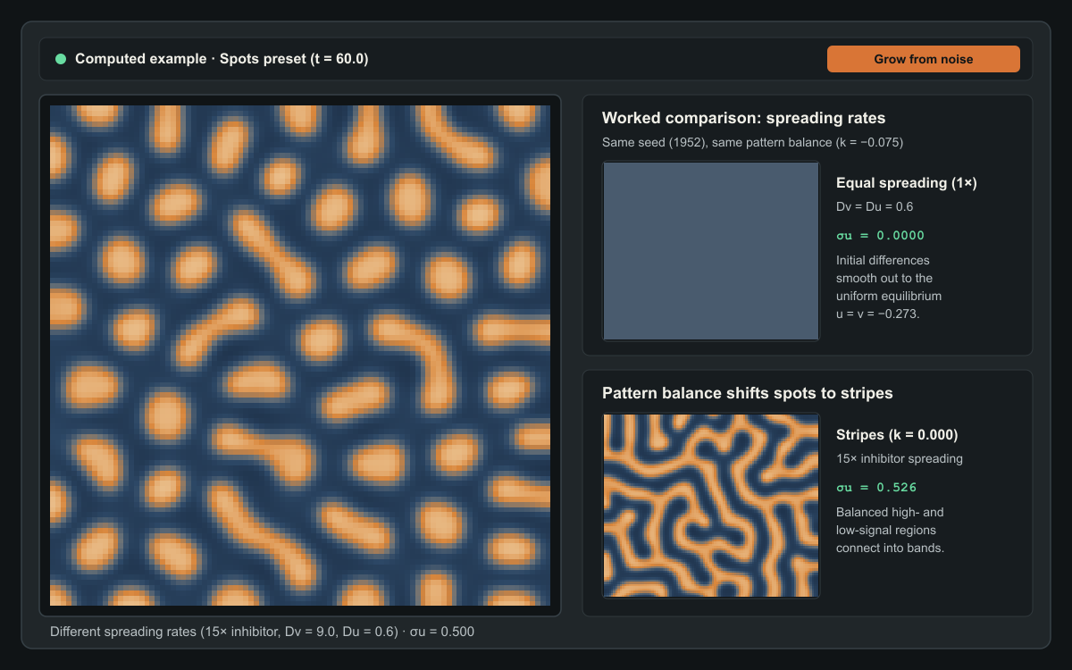
15× faster than the activator (D_u = 0.6, D_v = 9.0), tiny initial disturbances self-organise into isolated spots (k = −0.075), connected stripes (k = 0.000), or inverse spots (k = +0.075). Repeating the experiment at equal spreading rates (1×, D_v = D_u = 0.6) causes every disturbance to fade away.Computed example. Press Grow from noise to see how it forms.
How a nearly uniform surface develops spots or stripes
This computed preview compares the three verified Turing regimes at model time t = 60.0 from the same initial seed (1952, Grid 96 × 96,
spacing h = 0.8, inhibitor spreading 15× faster than activator
spreading, D_u = 0.6, D_v = 9.0) against an equal-spreading control
(1×, D_v = D_u = 0.6). When both signals spread at the same rate,
initial disturbances fade back to a flat equilibrium.
Three short suggested experiments
- Grow a pattern from microscopic noise: Leave the preset on Spots and press Grow from noise. The patch resets to tiny seeded disturbances () around its uniform equilibrium (). Watch local peaks reinforce themselves whilst fast-spreading inhibition carves quiet moats around each rising spot.
- Test equal spreading side by side: Select Compare equal spreading. Both fields restart from the exact same initial arrays and evolve at the same model time, changing only the inhibitor spreading rate (
15×on the left versus1×, where , on the right). Follow the spatial variation curve : differences amplify on the left and smooth to zero on the right. - Shift the pattern balance and domain geometry: Try Stripes () and Inverse spots (), or drag Pattern balance yourself. Then open Change the shape to compare a Broad sheet, a Narrow strip, and a Tapered patch, or switch to the Pigment view to see how a simple display threshold turns a continuous signal into crisp markings.
How local amplification and fast inhibition break symmetry
Everyday intuition says that diffusion is a smoothing process. Drop ink into still water and sharp edges blur until the liquid is uniform. For decades, biologists assumed that spatial patterns on animal coats—leopard rosettes, zebra stripes, or the dappled flanks of a trout—required either a pre-existing coordinate map or an external wave moving across the embryo.
Turing discovered a counter-intuitive exception. Suppose every point on a flat sheet carries two interacting signals:
- An activator signal () that promotes more of itself locally and also stimulates the production of an inhibitor.
- An inhibitor signal () that suppresses the activator and spreads through the sheet much faster than the activator does.
Imagine a nearly uniform surface sitting at equilibrium, perturbed only by tiny random fluctuations. Wherever the activator happens to sit slightly above the baseline, local self-amplification nudges that peak higher. At the same time, the growing peak produces extra inhibitor .
Because the activator spreads slowly (), the upward push stays localised in a tight cluster. Because the inhibitor spreads rapidly ( at the 15× setting), the newly created inhibitor escapes the nascent peak and floods its immediate surroundings. The peak survives at its own centre—where self-amplification outpaces the escaping inhibitor—whilst a ring of high inhibition around it prevents another peak from rising too close by. Farther away, where the inhibitor has diluted, another activator peak is free to grow.
The result is a characteristic wavelength: peaks space themselves out at a distance set by the contest between local amplification and the reach of the faster inhibitor.
Why equal spreading destroys the pattern
When you turn on Compare equal spreading, the second viewport runs the identical equations from the exact same initial arrays, but sets the inhibitor spreading rate equal to the activator spreading rate:
Why does the pattern vanish instead of merely changing size?
When both signals spread at the same rate, any inhibitor generated by a rising activator peak remains bottled up inside the peak itself rather than running ahead into the surrounding neighbourhood. As soon as rises at a point, rises right alongside it at the same spatial scale and quenches the peak on the spot. Meanwhile, ordinary diffusion smooths out local differences between neighbouring cells.
Without a faster inhibitor to export restraint outward, no spatial wavelength enjoys positive growth. Every disturbance decays steadily back towards the flat equilibrium , and the spatial variation drops to zero. Crucially, the workbench uses a fixed colour scale () across both fields and throughout playback; automatic contrast stretching would artificially amplify microscopic residual noise and make a fading surface look patterned when it is actually flat.
From spots to stripes and inverse spots
A faster inhibitor is necessary for pattern formation in this two-signal system, but it is not the only ingredient that decides which pattern appears. The Pattern balance parameter shifts the baseline drive on the activator signal and determines whether high-signal regions remain isolated islands or link up into continuous bands:
- Spots (): The uniform equilibrium sits below zero (). High-activator peaks face a headwind across the domain, so only compact, circular islands can sustain themselves amidst a connected low-signal sea.
- Stripes (): The equation is symmetric around . Neither positive peaks nor negative troughs enjoy an advantage; high- and low-signal regions share the surface equally (
~50%each) and weave into labyrinthine stripes of uniform width. - Inverse spots (): The uniform equilibrium sits above zero (). Now the high-activator state forms a connected background sheet punctuated by isolated low-signal pockets—the mirror image of the spots regime.
Whenever you adjust Pattern balance or Inhibitor spreading rate, the instrument restarts from the same deterministic random seed (1952 by default) so that differences you see on screen come purely from the equations rather than a fresh roll of random noise.
Signals versus visible pigment
A reaction–diffusion system produces smooth, continuous fields of and . In this dimensionless model, and are normalised, signed signal fields measured relative to a reference state: positive values represent above-baseline signalling and negative values represent below-baseline signalling. Unlike raw chemical concentrations, negative numbers here are completely valid.
In biological skin or hair follicles, downstream cells often respond to such continuous morphogen gradients through a sharp switch: where the activator signal sits above a threshold, pigment cells produce dark melanin; where it sits below, they produce light coat colour.
The three view tabs directly above the canvas let you separate the underlying mathematics from that readout rule:
- Activator and Inhibitor display the continuous signed fields and against a fixed scale.
- Pigment applies a binary threshold rule to . Moving the Pigment threshold slider changes only how the current field is coloured on screen; it never alters the numerical arrays, model time, or simulation state.
How patch geometry shapes the pattern
Open Change the shape to solve the exact same equations—with the same grid spacing () and diffusion coefficients—inside three flat, two-dimensional domains with no-flux boundaries (the signals spread inside the patch; they do not cross its edges):
- Broad sheet (
76.8 × 76.8model units): Large enough in both directions to host many wavelengths, producing isotropic spots or winding labyrinthine stripes. - Narrow strip (
96.0 × 19.2model units): Wide enough along its length for multiple waves, but narrow across its height. Because no-flux boundaries require signal gradients to meet the edges perpendicularly, stripes frequently align into rungs across the strip. - Tapered patch (
96.0 × 38.4model units): A flat two-dimensional wedge that narrows from left to right. At the broad end, two-dimensional spots or branched stripes can sit side by side; towards the narrow tip, only single transverse bands fit across the width—mirroring the transition from body spots to tail rings seen on cheetahs, genets, and leopard geckos.
Keep in mind that all three domains here are flat, two-dimensional approximations on a fixed grid. Modelling curved three-dimensional animal surfaces or tissue that expands while the pattern is still forming requires additional geometric terms beyond a fixed planar mesh.
Equations and implementation details
The instrument integrates the dimensionless cubic activator–inhibitor system on a two-dimensional domain :
Here and are normalised, signed signal fields where negative values are valid deviations below the reference baseline:
- : activator signal.
- : inhibitor signal.
- : local self-amplification () with a cubic limiting term () that keeps growing peaks bounded.
- : local inhibition of the activator by the inhibitor.
- : pattern balance parameter shifting the baseline drive on .
- : fixed activator diffusion coefficient.
- : inhibitor diffusion coefficient, controlled via the spreading ratio (so
1×means , and15×means ).
Uniform equilibrium and seeded initialisation
Setting and yields , where the uniform equilibrium satisfies the depressed cubic:
Because the derivative is strictly positive for all real , every pattern balance has a unique real uniform equilibrium solved analytically via Cardano’s formula. Each run initialises around using deterministic Mulberry32 pseudo-random disturbances of amplitude . Controlled comparisons reuse the exact same disturbance offsets at every grid cell.
Linear dispersion check and numerical discretisation
Linearising around gives the Jacobian reaction rates , , , and . For , the homogeneous mode () is stable because and . When , every spatial wavenumber also has . At (15×), a band of discrete Neumann eigenmodes on the grid () acquires positive growth rate with peak growth near (wavelength model units).
Spatial derivatives use a five-point finite-difference Laplacian with uniform spacing and zero-flux Neumann boundary conditions across all domain masks. Time integration uses the explicit second-order Heun (RK2) predictor–corrector scheme with fixed dimensionless timestep inside a dedicated Web Worker. Halving from to up to changes the field by less than RMS with cell-by-cell sign agreement.
Sources and further exploration
- Alan M. Turing (1952), The Chemical Basis of Morphogenesis, Philosophical Transactions of the Royal Society of London B, 237(641), 37–72.
- James D. Murray (1981), A Pre-pattern Formation Mechanism for Animal Coat Markings, Journal of Theoretical Biology, 88(1), 161–199, and Mathematical Biology II: Spatial Models and Biomedical Applications (Springer, 2003).
- Shigeru Kondo and Takashi Miura (2010), Reaction-Diffusion Model as a Framework for Understanding Biological Pattern Formation, Science, 329(5999), 1616–1620.
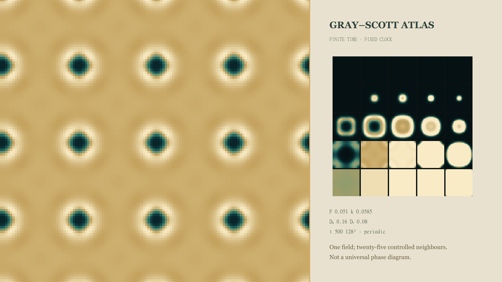
- Once you have explored how differential spreading creates spots and stripes in this signed activator–inhibitor model, visit the companion Gray–Scott Reaction–Diffusion Atlas on this blog to explore self-replicating mitosis spots, coral mazes, and spiralling waves across a two-parameter feed-and-kill phase map.
Quick reference and FAQ
Two spreading signals can turn an almost uniform sheet into spots or stripes—provided the restraining signal spreads faster than the amplifying one.
Word Cloud
Related reading
Selected by shared topics and section, with closer publication dates breaking ties.

Comments
Read the conversation or leave a thought for review. Comments load when this section is in view.