Ink That Follows a Scent

By Suvro Ghosh · Published 6 November 2026 · Updated 6 November 2026

Paint an invisible chemical trail. Watch the particles respond.

Each particle wanders randomly. Sensing adds a small push towards stronger chemical.

1. 1 Watch particles gather around the initial source.
2. 2 Drag the source elsewhere.
3. 3 Paint a curved line of chemical.
4. 4 Compare sensing on and off using the same starting positions and random nudges.

How can a group look purposeful when each particle follows only a local rule?

Thousands of independent particles move through a prescribed 256 × 192 chemical landscape by combining unbiased random wandering with an optional local push up the chemical concentration gradient. In the computed comparison below (seed 2026, t = 14.0 s), both runs share the exact same starting coordinates and random nudges at every step; only chemical sensing differs.

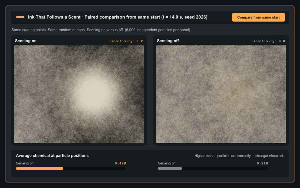
Model summary when canvas is unavailable: Each particle updates its position by nextPosition = reflectAtBoundary(position + sqrt(2 * D * dt) * randomVector + sensitivity * gradient(C, position) * dt). The chemical landscape is drawn directly on a fixed scale; this version does not simulate chemical spreading or decay.

How it works

The chemical landscape is drawn directly. This version does not simulate chemical spreading or decay.

At each fixed timestep (dt = 1/60 s), every particle updates its position independently on the fixed 256 × 192 logical domain using an additive biased random walk:

nextPosition = reflectAtBoundary(
  position + sqrt(2 * D * dt) * randomVector + sensitivity * gradient(C, position) * dt
)

• C (chemical concentration field): An invisible landscape on a fixed 0.0 to 1.0 scale, combining painted strokes on a smoothed 256 × 192 grid with an optional broad movable source peak.
• gradient(C, position): The local slope (∂C/∂x, ∂C/∂y) bilinearly interpolated at the particle’s current coordinate. Gradient magnitude is preserved (with a smooth stability cap for heavy painting) so steeper slopes pull more strongly than flat regions.
• D (random wandering): Controls the magnitude of the unbiased diffusive step sqrt(2 * D * dt).
• randomVector: Two independent standard normal values (Z_x, Z_y) generated deterministically from the tuple (seed, particleId, simulationStep, component).
• sensitivity: How strongly the local chemical gradient biases movement. Setting sensitivity to zero reduces the rule to a pure random walk.
• dt: The fixed simulation timestep (1/60 s), kept independent of display frame rate and browser resizing.
• reflectAtBoundary: Mirror reflection that keeps particles inside the 256 × 192 domain without wrapping lines across the canvas.

Chemical, particles, and trails remain separate: Chemical concentration is the environment; particles are independent point agents that read only their local surroundings; visible ink trails are a fading history buffer (512 × 384) that never attracts particles or deposits chemical. Clearing trails erases only the drawing, whereas clearing chemical removes the environmental pull while earlier marks fade naturally.

Why the paired runs share random nudges: In Compare from same start, matching particles in the Sensing on and Sensing off panels begin at identical coordinates and receive the exact same random nudge at every timestep. Because random walk noise cannot explain any divergence between the two panels, the visible separation isolates the effect of the local gradient-sensing term.

Teaching simplifications and scientific background: This experiment is a teaching approximation inspired by Chapter 11 of J. D. Murray’s Mathematical Biology I: An Introduction (Springer chapter reference), which connects microscopic biased random walks to macroscopic diffusion and chemotaxis. It does not model a specific biological organism, receptor adaptation, cell-to-cell signalling, nutrient consumption, chemical secretion, or physical chemical diffusion.

How can thousands of wandering particles gather around a shape they cannot see?

Start with a single patch of chemical. Each particle moves randomly, but sensing adds a small push towards a stronger concentration. Over time, more particles gather around the patch. Their trails make that influence visible.

Move the source to the other side of the canvas. The particles begin responding to its new position. The old marks remain for a while, so you can see the difference between where particles have been and where they are moving now.

Then try painting a curve.

The chemical itself is hidden. As particles encounter its slopes, their movement becomes biased towards the painted region. A drawing gradually appears through the accumulation of their paths.

They will not necessarily follow the curve from one end to the other. They respond to the chemical near their current position. That can bring them towards the curve and keep more of them nearby, without giving any particle a route to follow.

The comparison makes the effect easier to examine.

Choose Compare from same start. Both runs begin with the same particle positions, and each matching particle receives the same random nudge at every step. One run also responds to the chemical. The other has sensing switched off.

Watch how their paths separate.

Sharing the random nudges makes this a more useful comparison: a different sequence of random movements cannot explain the difference between the two runs. The sensing rule is what changes.

You can also switch sensing off during exploration. The particles continue wandering, and the earlier drawing takes time to fade. Turning off a rule changes what happens next; it does not remove the history of what has already happened.

That distinction matters throughout the experiment. Chemical is the environment the particles respond to. Trails record their movement. Clearing the drawing leaves the chemical intact. Clearing the chemical removes its influence while previous marks remain visible.

The coordinated appearance comes from many particles responding independently to the same surroundings. There is no leader, and the particles do not exchange messages.

This is a simplified way to explore chemotaxis: movement influenced by a chemical gradient. The chemical landscape here is prescribed directly. The model does not include chemical secretion, nutrient consumption, or the details of how a particular organism senses its environment.

The connection is to Chapter 11 of J. D. Murray’s Mathematical Biology I: An Introduction, which develops the relationship between random movement, diffusion, and environmental bias. The visualization uses those ideas in a small particle experiment. Read the chapter reference.

Paint something simple. Let the trails build. Then reveal the chemical field and compare it with the marks the particles have left.