The Epidemic Mosaic

By Suvro Ghosh · Published 7 November 2026 · Updated 7 November 2026

Two communities. One infection. Add a connection and see what changes.

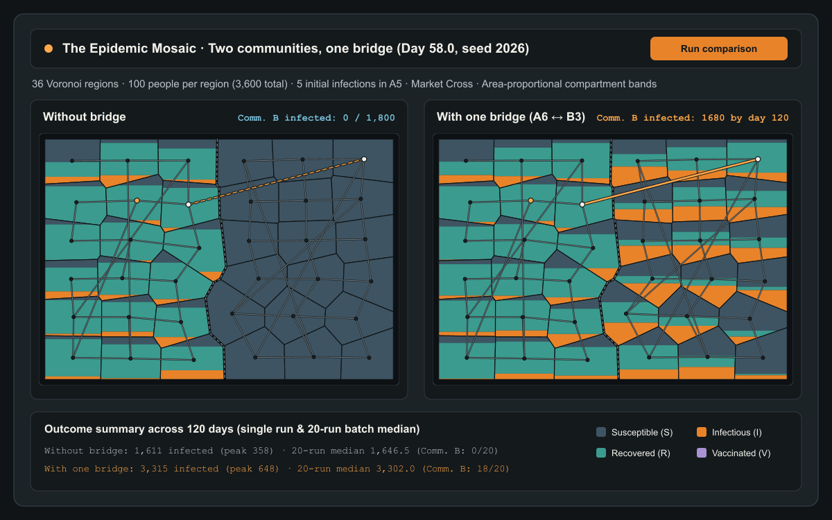
Each shape contains people. Lines show contact between regions. Sharing a border does not create contact.

Equal regional populations: Every region starts with 100 people (3,600 in total across 36 regions). Polygon size does not represent population.

Contact links, not migration: Edges represent contact opportunities between residents. People remain assigned to their home regions; this is not a model of physical travel or migration.

What changes when two separate communities gain one connection?

A reproducible synthetic city of 36 Voronoi regions (18 in Community A, 18 in Community B, 100 people per region) begins with 5 initial infections in A5 · Market Cross and none in Community B. Adding a single undirected bridge between A6 · Foundry Quay and B3 · Canal Basin allows transmission to cross between the communities without guaranteed spread on every run.

Note: This is a synthetic city for exploring transmission. It does not predict an outbreak in a real place.

What changes when two separate communities gain one connection?

Start with the default city above. Thirty-six irregular regions are divided into two communities of eighteen regions each: Community A on the left and Community B on the right. Every region holds 100 people, giving a total city population of 3,600. Polygon size does not represent population.

Five people begin infectious in A5 · Market Cross inside Community A. Everyone else in Community A is susceptible, and Community B begins without a single infection.

Press Run comparison.

Both scenarios start from day zero with the same city geometry, the same regional populations, the same five initial infections, and the same epidemic parameters. The only difference is one undirected contact link between A6 · Foundry Quay and B3 · Canal Basin.

Without that bridge, the infection can circulate along the contact links inside Community A, yet Community B must remain completely uninfected. With that single bridge in place, each infectious person in A6 · Foundry Quay creates a small daily hazard of infecting susceptible residents across the seam in B3 · Canal Basin. Once a single transmission crosses that link, Community B’s own internal contact network can carry the outbreak through the eastern half of the city.

Why borders and contact lines are separate

On an ordinary map, it is tempting to assume that two regions touch because they share a boundary. In this mosaic, geometry and contact network are kept deliberately separate.

Sharing a polygon border does not create contact. Look closely at A5 · Market Cross, where the infection starts: it shares long physical borders with A2 · Old Wharf and A8 · St Jude’s, yet no contact line joins them. Infection cannot pass directly across those borders. Conversely, A5 · Market Cross has a direct contact connection to A16 · South Downs near the foot of Community A. Visually distant regions can be one contact apart, and line length does not affect transmission strength.

Edges represent contact opportunities between residents. People remain assigned to their home regions; this is not a model of physical travel or migration.

Inside each polygon, horizontal colour bands show how the 100 residents are divided across states. Because Voronoi polygons narrow and widen from top to bottom, splitting a polygon by equal vertical height would distort the numbers. Here, the horizontal cuts are solved geometrically so that each band’s area matches its share of the region’s 100 people.

Four compartments in plain language

Before looking at the equations, the model tracks four groups of people in every region:

• Susceptible ($S_i$): People who have not had the infection and are not vaccinated; they can catch the infection from infectious people in their own region or across a drawn contact link.
• Infectious ($I_i$): People who currently have the infection and can pass it on before they recover.
• Recovered ($R_i$): People who have already had the infection and recovered; in this model they cannot catch it again.
• Vaccinated ($V_i$): People protected at day zero before the outbreak runs. Vaccination gives immediate, complete protection in this model, and is kept separate from recovery ($R_i$) so that cumulative infections count only people who were actually infected.

Experiment 2: With the same number of vaccine doses, does their placement change the outcome?

Switch the instrument to 2. Place the same vaccines.

The bridge between Community A and Community B stays fixed, and the five initial infections in A5 · Market Cross remain untouched. You are given a shared budget of 540 vaccine doses—15% of the city’s 3,600 residents—and three ways to place them at day zero:

1. Spread evenly: Allocate doses across all 36 regions, proportional to each region’s eligible susceptible population (15 doses per region).
2. Most connections: Prioritise the regions with the greatest total contact weight, concentrating protection in the network’s busiest hubs.
3. Around the bridge: Prioritise the two bridge endpoints (A6 · Foundry Quay and B3 · Canal Basin) and their directly connected neighbours.

Every strategy uses the exact same 540 doses. Yet when you run the comparison or inspect the Variation between runs (20 repetitions) panel, their behaviour diverges:

• Spreading 15% of doses evenly trims the outbreak modestly in both communities, but rarely stops transmission from crossing the bridge into Community B.
• Concentrating those same 540 doses in the most connected hubs substantially lowers the peak number of people infectious at once by dampening the highest-degree regions.
• Placing the 540 doses around the bridge endpoints and their immediate neighbours builds a local firewall across the inter-community bottleneck, keeping Community B uninfected across the 20-run ensemble at the default budget.

Neither targeted strategy is universally best under every network or parameter setting. If you raise the budget, move the bridge directly onto the initially infected region, or alter the ratio between within-region and cross-link transmission, the trade-off shifts.

Why repeated runs vary

Even when every parameter is held constant, a single stochastic run is only one possible history. With five initial infections, early recoveries can extinguish an outbreak before it leaves its starting region; in another run, early link transmissions can spark simultaneous chains in both communities.

Clicking Repeat 20 times runs the current comparison across 20 stored random seeds in a background Web Worker, retaining early extinctions alongside large outbreaks. The dot plot shows each individual run alongside the group median so you can see the variation between runs directly.

Mathematical model and allocation rules

For each region $i \in \{1, \dots, 36\}$, the simulation tracks integer counts

satisfying the conservation invariant

Each susceptible person in region $i$ experiences the instantaneous infection hazard

where $\beta_{\mathrm{local}}$ is the within-region transmission coefficient per day (default $0.28\,\text{day}^{-1}$), $\beta_{\mathrm{link}}$ is the transmission coefficient per unit-weight connection per day (default $0.04\,\text{day}^{-1}$), $w_{ij} \ge 0$ is the undirected contact weight ($1$ when a link is drawn, $0$ otherwise), and $\gamma = 1 / T_{\mathrm{inf}}$ is the recovery rate per day (default infectious period $T_{\mathrm{inf}} = 7\,\text{days}$). Adding a bridge inserts one undirected link of weight $w_{AB} = 1$ without normalising existing contact weights.

Events are simulated in continuous time using Gillespie’s direct method across three explicit event channels:

At each step, let $R_{\mathrm{tot}}$ be the sum of rates across all active channels. When $R_{\mathrm{tot}} > 0$, the waiting time to the next event is sampled as $\Delta t = -\ln(u_1)/R_{\mathrm{tot}}$ with $u_1 \sim \mathrm{Uniform}(0,1)$, and the specific channel is chosen with probability proportional to its rate using an independent uniform draw $u_2 \sim \mathrm{Uniform}(0,1)$. Because each link channel $(j \to i)$ is tracked separately, the simulation records the exact source and destination of every cross-region infection.

Deterministic integer vaccine allocation

At $t = 0$, region $i$ has eligible susceptible capacity $C_i = N_i - I_i(0)$ ($95$ in A5 · Market Cross and $100$ in all other regions, for a maximum city capacity of $3,595$ doses). Given a total integer budget $B \in [0, 3595]$, each strategy partitions the regions into priority tiers and distributes remaining doses within each tier using iterative largest-remainder (Hamilton) rounding subject to $0 \le V_i \le C_i$:

1. Spread evenly (even): All 36 regions form a single tier weighted by eligible capacity $C_i$. Ties in fractional remainders are broken by descending total contact weight $W_i = \sum_{j \ne i} w_{ij}$ and then ascending region index.
2. Most connections (most-connections): Regions are grouped into descending tiers of total contact weight $W_i$. Doses fill the highest-weight tier first (weighted by $C_i$, breaking remainder ties by shortest hop distance to the bridge and then ascending region index), overflowing into successively lower-weight tiers until all $B$ doses are placed.
3. Around the bridge (around-the-bridge): Let $d_i$ be the unweighted graph hop distance from region $i$ to the nearer bridge endpoint. Priority tier 1 comprises the bridge endpoints ($d_i = 0$, relative weight $1.5\,C_i$) together with their directly connected neighbours ($d_i = 1$, relative weight $1.0\,C_i$). Any budget remaining after saturating tier 1 overflows into shells $d_i = 2, 3, \dots$ weighted by $C_i \max(1, W_i)$ until all $B$ doses are allocated.

This is a synthetic city for exploring transmission. It does not predict an outbreak in a real place.

Inspired by J. D. Murray, Mathematical Biology I: An Introduction, Chapter 10 (Dynamics of Infectious Diseases): https://link.springer.com/chapter/10.1007/978-0-387-22437-4_10. For background on continuous-time Markov chain epidemic formulations and Gillespie simulation, see L. J. S. Allen (2017), A primer on stochastic epidemic models: Formulation, numerical simulation, and analysis.