The Fractal Atlas: A Field Guide to Infinity

Interactive Mathematics

A coastline with no country

A machine for zooming through the Mandelbrot set, breeding Julia sets, steering Burning Ships, mapping Newton’s quarrelsome basins, growing mathematical ferns and discovering how very small rules manufacture indecent quantities of geography.

⌖ centre −0.500000 + 0.000000i · span 2.800000

Enter the laboratory Take the five-minute tour

Runs locally in your browser. No API or account required.

PLATE 01 PARAMETER COAST

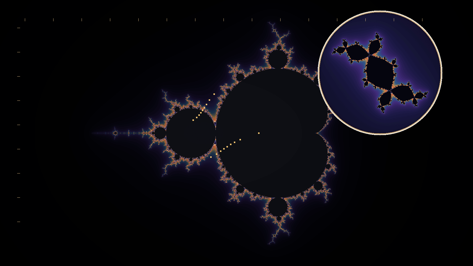
Most maps begin with a country and then worry about the coast. The Mandelbrot set begins with a rule small enough to fit on a bus ticket and somehow grows a coast that no computer can finish drawing. Every pixel is not painted. It is interrogated.

The interrogation is repetitive and rather bureaucratic. Square this number. Add that number. Do it again. And again. Some numbers bolt for infinity almost immediately. Some remain in the neighbourhood, circling, sulking, or settling into habits. Along the border between departure and apparent residence, the geography becomes absurdly elaborate.

The colours are not the fractal. They are the clerk’s notes in the margin: escaped after twelve rounds, escaped after eighty-seven, still here when the office closed.

Audio article

Uses the speech voice supplied by your browser or device.

The small machine beneath the scenery

The central machine is

Here $z$ is the current state. Squaring bends, stretches, and doubles angles in the complex plane. The parameter $c$ is added after every round. The answer becomes the next input. The resulting sequence

is called an orbit.

Iteration is the mathematical habit of putting the answer back through the front door. Imagine a municipal form whose final box says, “Copy this answer into Box 1 and submit again.” The smell of damp paper is optional; the feedback is not.

Feedback apparatus · ten rounds

Put the answer back

starting value→square→add c→new value ↖──────────────────────↙

A quick escapePeriod twoBoundary patience

Real part of c Imaginary part of c

Round 0 z₀ = 0 + 0i |z₀| = 0

Previous Feed it back Reset

Calculated orbit through the selected round

n	Re(zₙ)	Im(zₙ)	|zₙ|
0	0	0	0

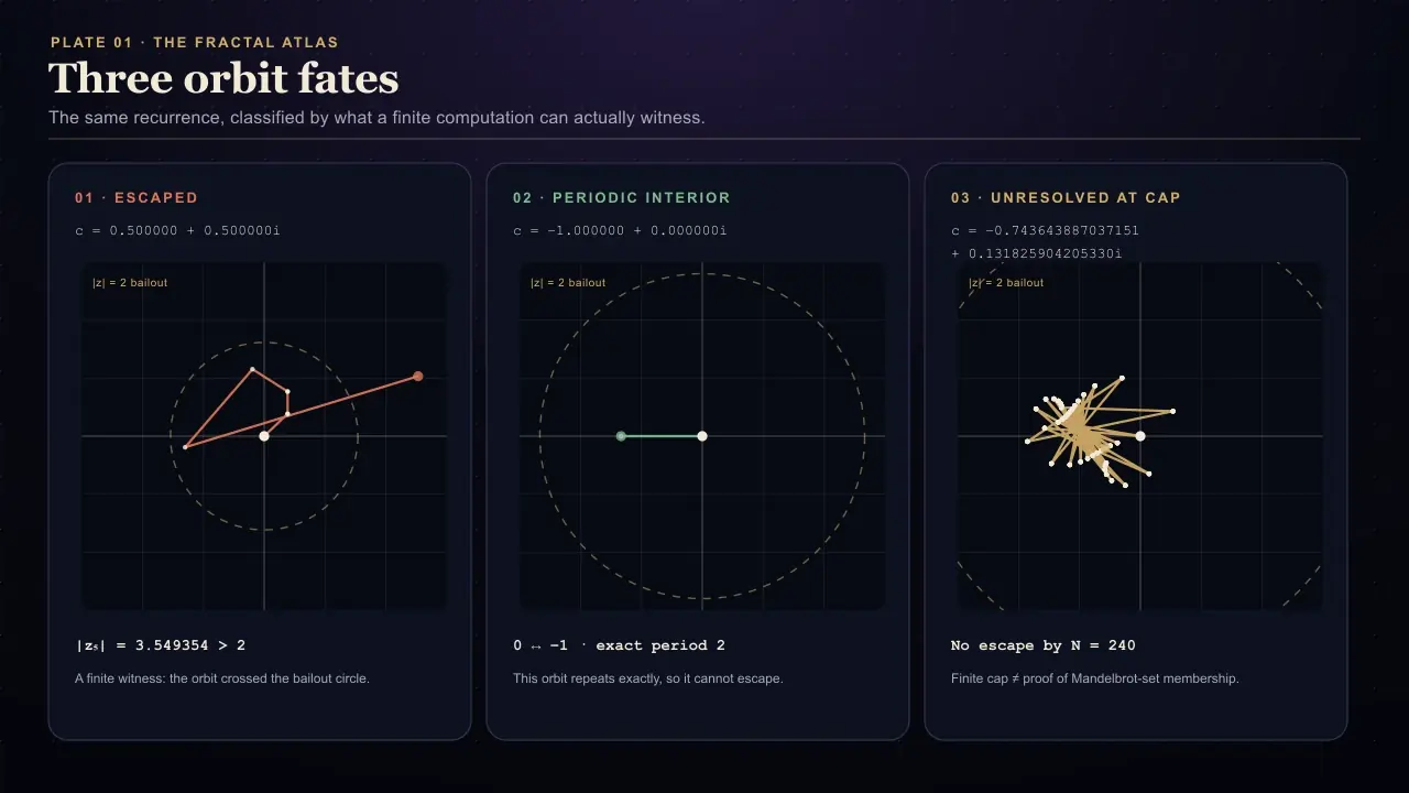
A computer performs this small loop for every pixel. It stops early when an orbit has unquestionably escaped, or it stops at the selected iteration limit and admits only that escape has not yet been observed. That distinction between bounded forever and not seen escaping yet is one of the atlas’s load-bearing ideas.

Complex numbers are addresses, not ghosts

A complex number

is an address with an east–west coordinate $a$ and a north–south coordinate $b$. The same quantity also has a magnitude and an angle. Multiplication combines scaling with rotation; squaring squares the magnitude and doubles the angle.

Drag the point below. The first mark is $z$, the second is $z^2$, and the third is $z^2+c$. Nothing supernatural has happened. One coordinate pair has been transformed, then translated.

Drag anywhere in the plane

Complex-plane transformer

One point, three addresses

Re(z) Im(z)

z

0.72 + 0.46i

|z|

0.854

angle

32.574°

z²

0.307 + 0.662i

fixed c

−0.55 + 0.28i

z²+c

-0.243 + 0.942i

Squaring doubles the angle. Adding c translates the squared point by one fixed complex address.

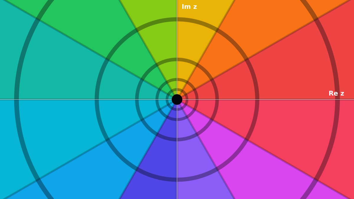
If you want to see how arbitrary complex functions can be mapped directly through hue and magnitude, the companion essay Every Complex Number Has a Colour treats that different experiment. Domain colouring maps the output of a function once. This atlas repeatedly feeds an output back into the same function and asks about its fate.

The Fractal Atlas laboratory

The instrument below is the common nervous system for the whole essay. Drag the map, zoom beneath the pointer, select a family, inspect an orbit, change its colours, or load a field expedition. Prose buttons elsewhere on the page operate this same laboratory rather than opening disconnected demonstrations.

Live field instrument · schema v1

The Fractal Atlas

escape time

↶ Undo ↷ Redo ⌂ Reset ↺ Reset all ＋ Zoom in − Zoom out ↗ Full

Quadratic pair

MandelbrotJulia

Altered recurrence

MultibrotBurning ShipTricornPhoenixMap Workshop

Convergence

Newton

Orbit traffic

Buddhabrot

Recursive cousins

Barnsley fernSierpińskiL-systems

Mandelbrot set zₙ₊₁ = zₙ² + c, z₀ = 0

Tap once to engage touch navigation. Drag to pan, scroll or pinch to zoom, double-click to zoom in, click or press Enter to inspect an orbit, and use the arrow or plus and minus keys to navigate. Press Escape to release touch navigation.

Linked Julia · c = -0.123 + 0.745i pixel → z₀ · c fixed

Pointer / pinned coordinate -0.123 + 0.745i

Centre -0.5 + 0i

Vertical span 2.8000e+0

Backend preparing

Preparing a bounded renderer…

Preparing the atlas instruments…

Family passport · Mandelbrot set zₙ₊₁ = zₙ² + c, z₀ = 0

Family passport

Mandelbrot set

Formula

zₙ₊₁ = zₙ² + c, z₀ = 0

Computational class

escape-time

The pixel represents

The parameter c

What stays fixed

The starting value z₀ = 0 and the quadratic rule

What changes

The parameter c changes from pixel to pixel

What the colour means

Whether the orbit escaped, and how quickly it did so

Typical symmetry

Reflection across the real axis

What to try

Probe points on both sides of the main boundary.

History and finite-computation note

Computer experiments made the connectedness map of quadratic Julia sets visible at useful scale.

Computer caveat: Not escaping before the iteration limit is evidence of unresolved boundedness, not a proof for an arbitrary pixel.

Read the corresponding field note

Navigation desk

Move, link and compare

Start guided tour

Drag to pan; Shift-drag draws a rectangular zoom. Wheel, double-click or pinch zooms beneath the pointer. Click a pixel to pin its orbit, or drag the pinned crosshair. Keyboard: arrows and +/− navigate; Alt+arrows move the crosshair one pixel (Shift+Alt moves eight); R, 0 or Home resets; H or [ returns to the previous view and ] moves forward; O toggles the Orbit Inspector (I also opens it); C and P open Colour and Presets; J links Julia; V compares; G toggles the grid; F toggles fullscreen; Escape releases touch navigation or closes the active overlay.

Coordinate gridAxes and scale marks Linked JuliaPreview c under the pointer Compare modeOne common instrument, two panes Analytic interior testsQuadratic cardioid and bulbs Cardioid + bulb guideAnalytic boundaries, clearly overlaid Degree symmetry guide1-fold parameter guide

Render quality battery saverdraftbalancedhigh

Exact viewport

Centre real · decimal string Centre imaginary · decimal string Vertical span

Copy exact centre Zoom 2× Zoom out 2×

Two nearby laws

Pinned Julia parameters

A

-0.123 + 0.745i

B

-0.124 + 0.744i

Δc

-0.001 − 0.001i |Δc| = 0.0014142135623730950488016887242096980785696718753769480731766797379907324784621070388503875343276415727350138462309122970249248360558507372126441214970999358314132226659275

Pin selected as A Pin selected as B Compare Julia A / B Build Julia path A → B

Pin A and B from the Mandelbrot plane, then compare their critical orbits by swapping the two Julia panes and opening Orbit.

The census and the citizen

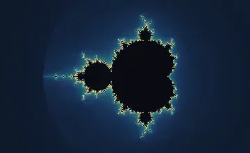
The Mandelbrot and Julia pictures often appear beside one another in books, as if they were cousins at a family wedding. Their relationship is much tighter. They are two questions asked of the same recurrence.

For the Mandelbrot set, every pixel supplies a different value of $c$. The starting value remains $z_0=0$. The map is a parameter plane: a census of possible laws.

For a quadratic Julia set, $c$ remains fixed. Every pixel supplies a different starting value $z_0$. The map is a dynamical plane: one law applied to an entire population of starting points.

In the Mandelbrot view, the pixel chooses the law. In the Julia view, the law is fixed and the pixel chooses where the experiment begins.

↗ Show the Julia set born from this point

In linked view, moving the pointer across the parameter plane updates a deliberately draft-quality Julia preview using the hovered value of $c$. Clicking pins that value. Drag the pinned crosshair and the companion follows at preview quality; releasing it pins the latest coordinate and requests the selected final quality. The primary plane likewise lowers its own resolution while it is being panned or pinched and refines when the gesture ends. The coordinate remains visible because “rabbit”, “Basilica”, and “dendrite” are useful nicknames only after the number has been supplied.

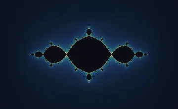
Try $c=0$. The filled Julia set is the unit disk. Try $c=-1$ and the Basilica appears. At approximately $c=-0.123+0.745i$, a rabbit-like period-three structure emerges. The atlas avoids pretending that an attractive but inexact parameter has acquired a certified historical name merely because its ears look cooperative.

The border does the interesting work

A point far outside the Mandelbrot set usually escapes quickly. A point in the main cardioid can be certified as interior by an analytic test. The expensive uncertainty gathers near the boundary, where two coordinates closer than one displayed pixel can have strikingly different orbit histories.

Escape is easier to prove than imprisonment. For the quadratic map, once $|z|$ exceeds the bailout radius $2$, the orbit cannot return. The computer has a certificate of departure. After 500 quiet rounds, by contrast, the honest sentence is:

After 500 rounds the computer has not seen it escape.

It may be inside. It may be a late escapee. It may sit in a numerically troublesome neighbourhood. A dark pixel is therefore a computed status under stated settings, not a stamped passport from infinity.

↗ Follow one escaping orbit

The orbit inspector exposes the selected coordinate, $z_0$, $c$, each calculated $z_n$, its magnitude, escape or convergence status, apparent period, and—where relevant—the root reached. The plotted path and HTML table describe the same values, so the Canvas is never the only witness.

The relatives who altered one line of the recipe

Change one operation and an entire continent reorganises itself.

Field classification

Several questions, one atlas

Escape-time maps

A pixel launches an orbit and the renderer asks whether it escapes.

Mandelbrot →Julia →Multibrot →Burning Ship →Tricorn →Phoenix →

Convergence basins

A pixel votes for the root reached by an answer-finding process.

Newton fractals →

Orbit density

Escaping routes accumulate into a histogram instead of one colour per parameter.

Buddhabrot →

Recursive cousins

Affine choices, removal rules, and grammars construct limiting objects.

Barnsley fern →Sierpiński →L-systems →

In a Multibrot, the square becomes an integer power:

The degree changes the symmetry of the parameter plane. The first version deliberately refuses non-integer powers; complex fractional powers require a branch convention, and a hidden branch cut is not a harmless implementation detail.

↗ Turn the square into a cube

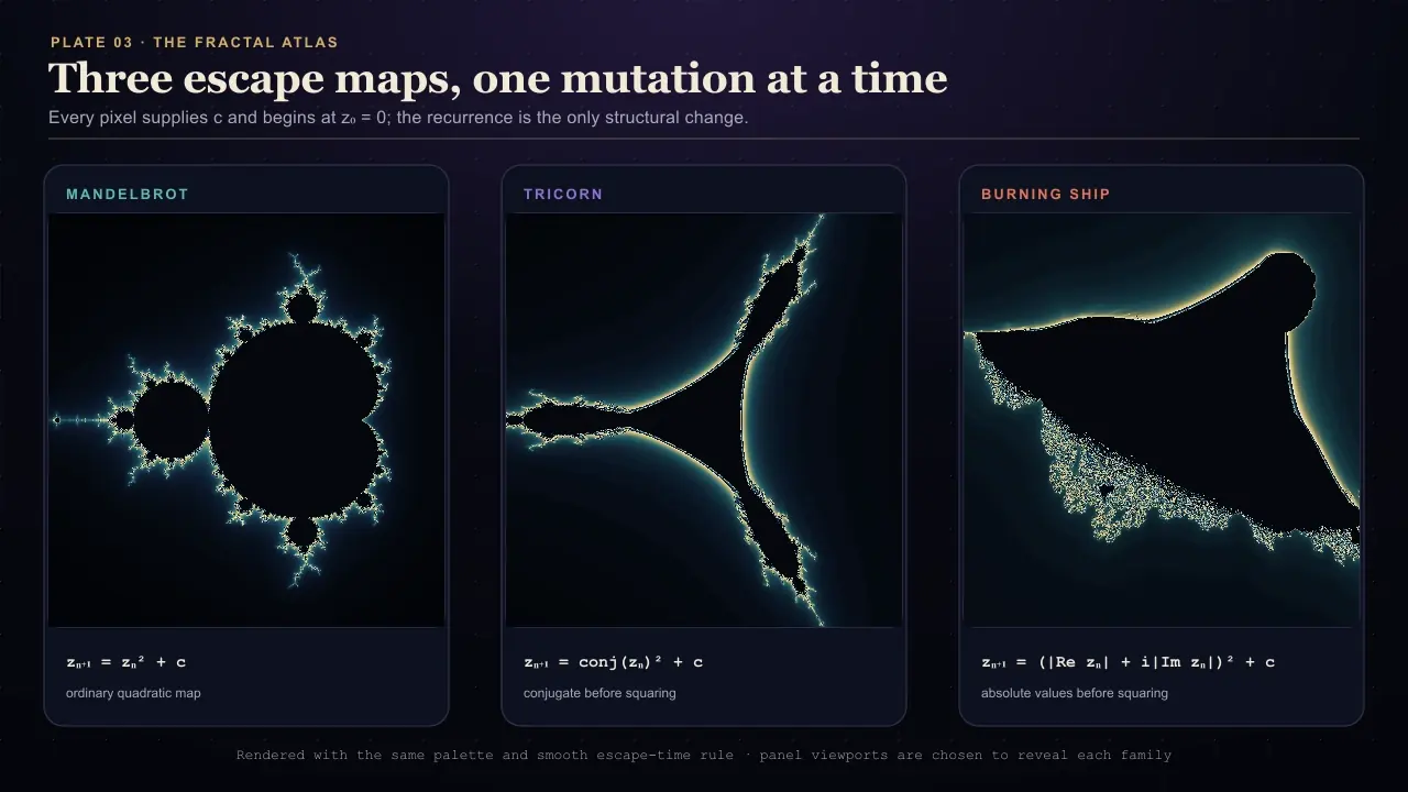
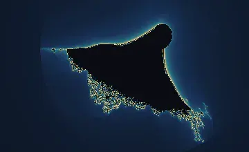
The Burning Ship takes absolute values before squaring:

That placement matters. The absolute values destroy the ordinary holomorphic structure; the result is not merely “Mandelbrot but pointier”. A visible presentation control may flip the finished view vertically, but it does not smuggle an unexplained inversion into the recurrence.

The Tricorn, also called the Mandelbar set, conjugates before squaring:

The conjugation turns a holomorphic iteration into an antiholomorphic one. The formula passport shows the bar explicitly instead of leaving the image to explain a changed operation by facial expression.

The Phoenix map remembers:

Most escape-time examples need only the current value. Phoenix carries the previous value into the next round. Its step table therefore has an extra column: memory deserves paperwork too.

The laboratory exposes both the complex memory coefficient $p$ and the initial remembered value $z_{-1}$. The ordinary preset begins with $z_{-1}=0$, but changing that value changes the first step of this genuinely second-order recurrence.

↗ Give the recurrence a memory

Newton draws a map by trying to solve an equation

Newton’s method was designed to find roots:

The relaxation parameter $\lambda$ defaults to $1$, which recovers the ordinary Newton step. Smaller values damp the correction; values up to the laboratory’s bounded maximum may over-relax it. Give every starting point in the complex plane its own vote, however, and the answer-finding procedure draws borders more intricate than the problem it was hired to solve. For $f(z)=z^3-1$, three roots divide the plane into three basins. Hue identifies the root reached; brightness or contours record how long convergence took. A neutral point means unresolved, non-convergent, or too close to a derivative singularity under the current calculation—not a secret fourth party.

↗ Let Newton choose among three roots

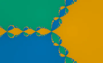
The coefficient editor constructs a bounded polynomial. It never executes a typed JavaScript expression. Roots, derivative values, tolerances, and iteration limits remain data with explicit bounds.

The colours are evidence, not paint

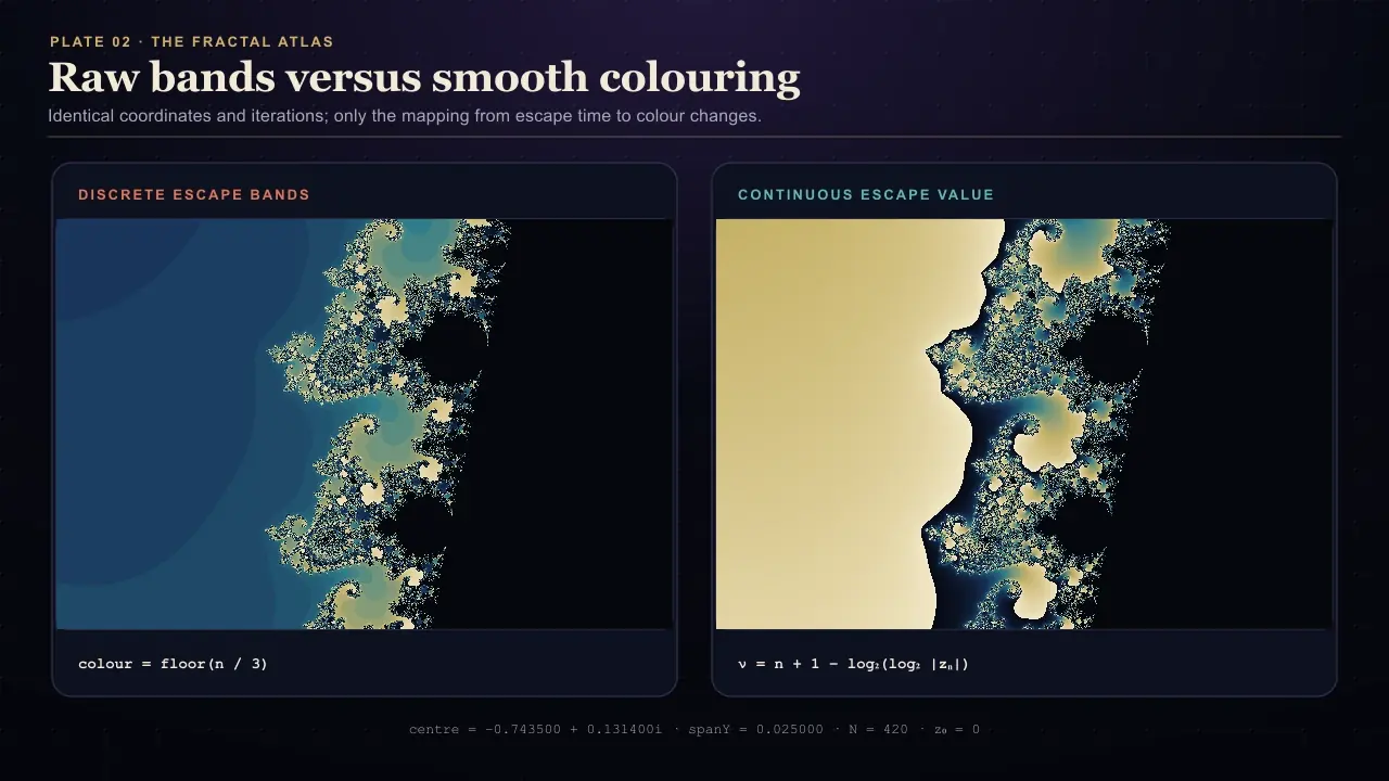
Escape-time colouring records how long the computer waited before giving up on an escaping orbit. Discrete bands show the integer count plainly. Smooth colouring estimates a fractional escape value so neighbouring counts do not form hard stripes. Distance shading and orbit traps encode other numerical evidence. Newton mode assigns families of colour to converged roots. Buddhabrot brightness records accumulated traffic.

None of these colours belongs to the fractal. The same computed field can wear several uniforms.

↗ Remove the colours

Binary mode is severe but clarifying: escaped versus unresolved or certified interior. Banded mode reveals the loop count. Smooth mode removes much of the clerical striping. Orbit traps ask how closely an orbit approached a point, line, circle, cross, or grid. A shaded distance estimate resembles relief, but the atlas labels it as a visual interpretation rather than three-dimensional terrain.

Palettes are deliberately inspectable. Stops, offset, cycle count, reversal, interior treatment, and root categories remain visible. Selected state and warnings also use borders, labels, symbols, or contours; hue does not have to carry the entire bureaucracy.

A colour ledger can change the question

Two pictures can use the same orbit calculation and still emphasise different evidence. Escape bands partition the result by integer waiting time. Smooth escape colouring estimates a value between those integers, making the transition less like a stack of contour cut-outs. Histogram equalisation goes further: it first counts the escape values present in the entire frame, builds their cumulative distribution, and then allocates more of the palette to crowded parts of that distribution.

That last method requires two passes. A renderer cannot correctly equalise a pixel from its orbit alone because the pixel’s colour depends on what happened everywhere else in the image. The atlas therefore completes a bounded frame census before applying the palette. It does not call ordinary smooth colouring “histogram mode” merely because the result looks pleasantly balanced.

Distance and trap methods change the ledger again. A distance estimate asks for an approximate distance from an escaped point to the boundary and relies on derivative information that is not valid for every recurrence. Burning Ship’s component-wise absolute values and the Tricorn’s antiholomorphic step break the simple complex derivative used by the ordinary quadratic map, so unsupported combinations are removed rather than decorated with a dubious number. An orbit trap does not estimate the boundary at all; it records the closest approach to a chosen geometric object.

Newton basins need categorical colour before they need a gradient. One root should keep one identity even when brightness records convergence speed. Interpolating between “root red” and “root blue” would invent a fourth political party that the polynomial never elected. The palette laboratory therefore distinguishes continuous ramps from discrete basin categories.

Where the computer begins to lie

The screen is not infinity. It is a finite agreement among four limits that are often confused.

First, a Canvas has finitely many pixels. Each pixel covers an area of the complex plane even if the shader samples one representative coordinate. Second, the loop has a finite iteration limit. A late escape can remain unresolved at 300 rounds and escape at 2,000. Third, floating-point numbers have finite precision. Deep enough into a zoom, adjacent pixels can become the same representable coordinate. Fourth, the renderer may lower resolution temporarily while a gesture is in progress, then refine after the gesture ends.

More iterations help only the second problem. They cannot distinguish coordinates that arithmetic has already collapsed. More colour bands help none of them.

↗ Take me to where arithmetic runs out of road

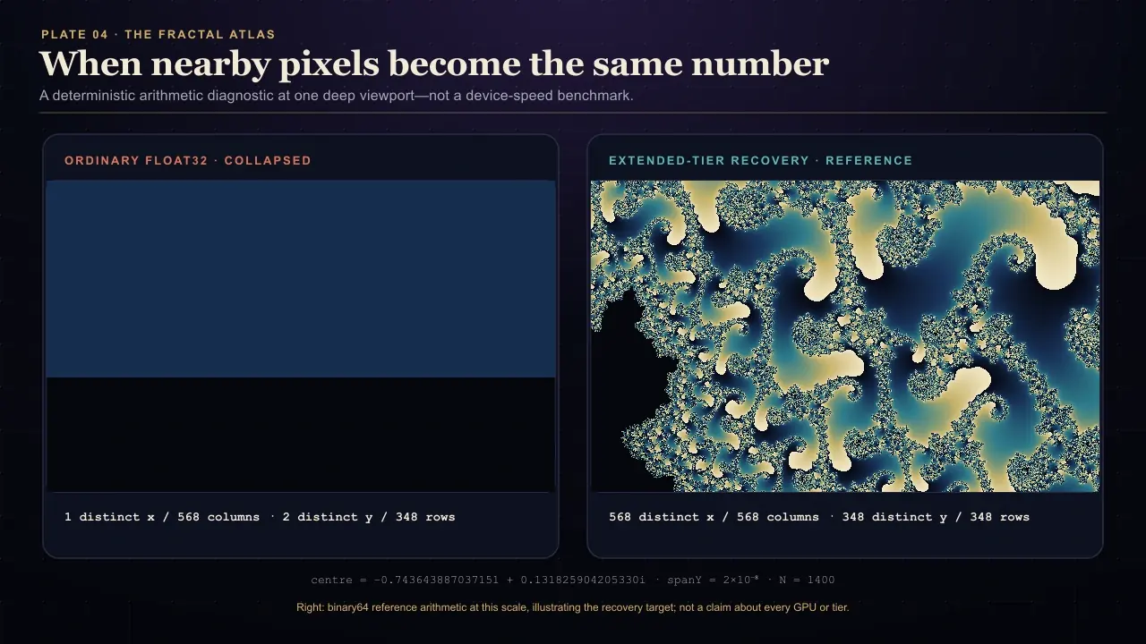
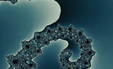
The precision meter reports centre, span, approximate magnification, renderer, and whether neighbouring device pixels still produce distinct represented coordinates. “Comfortable”, “Approaching limit”, and “Precision exhausted” describe the calculation, not the set. Ordinary views use high-precision GPU floats. When their coordinate grid collapses, the standard quadratic Mandelbrot and Julia paths can use tested double-single arithmetic: every important value is a high-and-low pair, and the shader carries those pairs through coordinate mapping, complex addition, and complex multiplication.

The published laboratory stops at that tested double-single tier. Its verified battery-saver diagnostic view uses a vertical span of (2.4\times10^-13) at 240 iterations and a 234 × 198 render target inside a 900 × 700 browser viewport—about (1.2\times10^-15) complex units per device pixel, or roughly (1.17\times10^13) magnification from the default view. Smaller URL coordinates are still preserved as Decimal strings for sharing and orbit inspection, but the fallback raster is labelled CPU double and the meter is allowed to say Precision exhausted.

There is a bounded quadratic perturbation research path in the source: it calculates a decimal reference orbit in a cancellable worker, diagnoses samples, rebases to a small reference grid, uploads double-single coefficient pairs, and advances relative GPU deltas. It is deliberately not enabled in the published runtime. On the target Chrome/ANGLE stack, compiling that driver shader synchronously blocked the page for well over 45 seconds; the uploaded coefficients also require wider cross-GPU validation before they deserve a public deep-zoom claim. The atlas therefore follows the less glamorous but correct rule: preserve the coordinate, disclose the collapse, and do not paint unverified detail. Other families likewise stop at their honestly reported double or double-single ceiling. None of these devices turns a finite screen into “infinite zoom”.

The WebGL2 renderer is feature-detected and event-driven. It draws when state changes and stops when the picture is complete. If WebGL2 is unavailable, a bounded Canvas 2D path preserves Mandelbrot and Julia navigation and numerical inspection at a lower resolution. Progressive density and point-cloud work uses a worker where supported. WebGL2 and OffscreenCanvas are useful browser facilities, not universal magic carpets. Hello, Fragment opens the underlying GPU idea one pixel at a time, while the Visualizations gallery leads to the site’s other live mathematical instruments.

The ghost made by escape

The ordinary Mandelbrot image asks which parameters stay. The Buddhabrot draws the traffic left by parameters that eventually escape.

The worker samples $c$, calculates the usual critical orbit, rejects candidates that do not escape within the chosen limit, and accumulates the visited positions of escaping orbits into a histogram. Exposure and gamma turn that histogram into visible density. Three iteration windows can feed red, green, and blue channels for a Nebulabrot view.

↗ Draw the traffic of escaped points

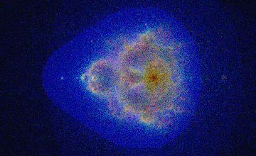
The seed, bounds, sample budget, and settings determine the run. Pause and resume change when work occurs, not which deterministic sequence is eventually accumulated. The progress strip distinguishes candidate samples, accepted escaping orbits, plotted orbit points, and display pixels. Noise is not concealed as mysterious celestial fog; it is finite sampling.

A fern assembled by probability

The recursive cousins belong in the atlas because they expose a different route from small rules to large geography. They are not squeezed into the escape-time family merely to inflate the guest list.

A Barnsley fern uses several affine photocopiers. One compresses a point into the stem. Others rotate, shrink, shear, and move it into parts of the leaf. At each step, one map is selected with a stated probability. The fern is not traced from stem to tip. A single point is repeatedly relocated, and the leaf appears statistically from the accumulated visits.

↗ Grow the fern one toss at a time

A seeded random source makes the same sequence reproducible. Slow mode reveals the active affine transform. Progressive mode spends a bounded point budget. Advanced controls expose the transformation table without accepting executable code.

The Sierpiński triangle arrives by two roads. A chaos game repeatedly moves a point halfway towards a randomly selected vertex. Recursive removal begins with one solid triangle, removes the central triangle, and repeats the instruction on the three survivors. The procedures look unrelated, yet they reveal the same limiting object.

An L-system rewrites a restricted grammar and asks a turtle to walk the result. Koch, dragon, Hilbert, snowflake, and plant presets expose axiom, production, generation, angle, step, line thickness, and depth colour. Before expanding, the laboratory estimates the symbol and segment count, warns at high cost, and applies a hard ceiling. SVG export is offered only while the construction remains genuinely vector-sized.

The fern’s seeded sampling has a useful neighbour in The Casino That Calculates, where statistical error is the subject rather than a drawing material. For another system in which small local rules accumulate into a changing population, visit the Artificial Life Lab. And if the interesting part is the GPU as an evolving artistic medium, Create Art: A Living Pigment Studio follows pigment, moisture, motion, and drying instead of complex orbits. All three are browser models, but each makes a different promise about what its pixels mean.

Similarity is a family resemblance, not a rubber stamp

“Self-similar” is often used as if it meant “contains tiny photocopies of itself everywhere”. The Sierpiński triangle comes close to that strict picture: each surviving triangle is an exact scaled copy of the whole construction. A Koch curve also repeats an exact replacement rule. Their similarity is built into the recipe.

The Mandelbrot boundary is subtler. Magnified regions frequently echo bulbs, spirals, antennae, and miniature copies of the whole set, but the surrounding arrangements and scales change. The useful phrase is quasi-self-similarity: related motifs recur without turning every neighbourhood into an exact tiled copy. A Julia set can be locally intricate for the same dynamical reason while looking globally unlike the parameter plane that selected its value of $c$.

The fern introduces statistical self-similarity. Its affine maps send the accumulated cloud into smaller leaflets with related distributions, yet the displayed points depend on a finite seeded sample. A different seed changes which particular dots appear first, not the limiting distribution prescribed by the transformations and their probabilities.

This is also why “fractal dimension” needs a question attached. A box-counting estimate asks how the number of occupied boxes changes as the box size shrinks. Hausdorff dimension is a deeper mathematical definition and is not generally obtained by fitting a line through a few screen resolutions. Topological dimension, area, boundary dimension, and the dimension of a plotted finite point cloud need not answer the same question. The atlas does not manufacture a decimal dimension badge from one raster and present it as a theorem.

The common thread is not a single visual texture. It is the production of structure across scales by iteration, recursion, replacement, or repeated selection. That is enough to place these constructions in one field guide while still preserving the differences among escape maps, convergence basins, density accumulations, and recursive cousins.

Field expeditions

Random coordinates are usually dull. The atlas therefore carries named, tested expeditions with a question attached.

↗ Take me to Seahorse Valley

At the whole-set view, notice the cardioid and bulbs before zooming. Across a boundary, click one parameter and pin it as A, then click a nearby parameter and pin it as B. The atlas can place the resulting Julia laws side by side; its orbit instrument examines the primary law and one selected starting point at a time, so swap A and B to compare corresponding rows sequentially rather than expecting a simultaneous two-orbit table. In Seahorse Valley, increase iterations without confusing patience with proof. In the Basilica and rabbit-like Julia examples, keep the law fixed and change starting points. Then change the law itself: degree three, Burning Ship, Tricorn, Phoenix, or Newton.

The guided tour performs the same sequence for a first visit: pixel, feedback, escape, boundary, linked Julia, altered operation, convergence basin, and recursive cousin. It preserves the pre-tour state, permits back and skip, avoids trapping focus, and replaces animated travel with direct state changes under reduced motion.

Saved specimens remain on this device. A specimen contains its family, viewport, parameters, palette, seed, and a schema version. The URL stores bounded readable state for a permanent link; invalid or extravagant values are rejected before they can allocate enormous buffers or launch an absurd render. Browser Back and Forward restore meaningful committed views while pointer movement and live dragging replace only the current history entry.

PNG and settings JSON exports are local. The current composed PNG includes the visible grid and pinned selection marker. The orbit inspector’s path and table remain in their own instrument; they are not painted over the main map or added to this PNG. For supported raster families, 1×, 2×, 4×, and custom exports instead re-sample the unadorned target image in seam-free tiles, yielding between them so the page remains cancellable. Before starting, the instrument states pixel count, estimated peak memory, and the effective iteration count after its work budget. It will lower an extravagant iteration request or reject unsafe dimensions rather than invite a tab crash.

Histogram equalisation stays with the current composed frame because a tiled approximation without a global cumulative distribution would be false advertising. Progressive point clouds likewise export their accumulated visible state. Suitable recursive curves may export SVG only below the safe segment limit; once a construction becomes too large, raster is the honest container. Shader fields do not pretend to be vectors.

The humans before the pixels

The history did not begin when colour monitors became attractive. Around the beginning of the twentieth century, Pierre Fatou and Gaston Julia independently investigated what repeated rational functions do to the complex plane. Their questions concerned stability, exceptional behaviour, and the boundaries between kinds of motion; they were not instructions for a screen saver. In 1918 Julia published a long memoir on rational iteration. The original journal record lists pages 47–245, a useful antidote to the idea that his contribution was merely the later picture carrying his name. Modern terminology commemorates both mathematicians: the Fatou set describes regions where nearby iterations behave stably in a technical sense, while the Julia set is the boundary of that stability. The clean black-and-gold raster came much later.

Several lines of mathematics and computation then converged on quadratic parameter space. Benoît Mandelbrot brought a sustained interest in rough geometry, scaling, and visual evidence to the subject. His long tenure at IBM gave him access to unusual computing resources and colleagues at a time when drawing repeated complex arithmetic was itself substantial work. Parameter-space images associated with his work around 1980, followed by the 1982 book The Fractal Geometry of Nature, helped make fractal geometry visible far outside a specialist circle. IBM’s account of that setting emphasises the role of computer graphics and the research environment. It is still more accurate to describe Mandelbrot as a powerful investigator, synthesiser, namer, and populariser than as the solitary inventor of everything now filed under “fractal”.

Adrien Douady and John Hubbard supplied another decisive thread: rigorous complex dynamics connecting the parameter plane to the many Julia dynamical planes it organises. Their work in the early 1980s developed tools for understanding the Mandelbrot set’s topology and proved, among other results, that the set is connected. The surviving Orsay notes in English say that they present results obtained in 1981–82 and grew from Douady’s later course notes. The result matters visually: the black set is not an accidental heap of disconnected islands, even though a finite, poorly sampled raster may make thin connections impossible to see. Douady and Hubbard’s theory also made external rays and the relationship between parameter behaviour and dynamical behaviour into instruments of proof rather than picturesque analogies.

Home computers subsequently made fractals celebrities: demo-scene feats, album covers, wallpaper, and occasionally mathematical kitsch. At first, deeper zooms could be bought mainly with more iterations, more precision, and more waiting. Arbitrary-precision arithmetic pushed past the range of ordinary hardware numbers but became expensive when repeated independently for every pixel. Later deep-zoom renderers learned to compute one high-precision reference orbit and express nearby pixel orbits as perturbations of it; series approximations could skip blocks of common early work. A widely circulated 2013 technical note on Mandelbrot perturbation explains both the economy and the need to notice when a chosen reference is no longer trustworthy. Glitch tests, rebasing, and additional reference orbits are engineering safeguards, not proofs of infinity. Decoration is not the enemy. The trouble begins when a palette or a heroic zoom hides the numerical method that produced it.

What the picture does not prove

An image is evidence of a calculation, not a proof of the infinite object. A finite iteration can leave a pixel unresolved. Floating-point arithmetic can merge nearby coordinates. A palette can manufacture a sharp-looking contour in a smooth numerical field. Approximate period detection depends on tolerance. A beautiful render can be numerically poor.

The atlas therefore ends with a concrete experiment instead of a sermon. Return to a complicated Mandelbrot boundary and choose a point on each side of a thin colour transition. Pin the first as A and the second as B, recording $\lvert\Delta c\rvert$. Open Compare Julia A / B. In the primary Julia plane, select one starting point $z_0$ and note the first several orbit rows and the reported status. Swap A and B, keep the same $z_0$, and inspect those rows again. Then raise the iteration budget once without changing either coordinate. Ask four precise questions: did the law change, did the starting point change, did only the observed status change, and did the precision meter still distinguish neighbouring pixels?

These pictures do not arise because equations contain hidden illustrations. They arise because feedback magnifies tiny differences, and the map of those differences becomes a geography.