Complex Functions as Landscapes: A 3D Domain-Colouring Laboratory

Audio article

Uses the speech voice supplied by your browser or device.

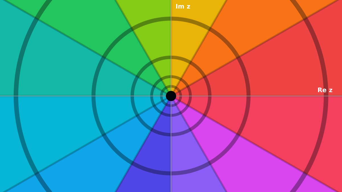
Four coordinates, one honest compromise

Write the input to a complex function as

and its output as

The full graph therefore consists of points $(x,y,u,v)$ in four-dimensional real space. A screen cannot place all four coordinates along three spatial axes. Adding depth does not uncover a hidden “imaginary dimension”, and it does not make the whole complex function suddenly visible. Something must still be omitted or carried by colour, contours, labels, or a second coordinated view.

This laboratory makes that compromise explicit. The ordinary landscape uses $\operatorname{Re}z$ and $\operatorname{Im}z$ as the two horizontal directions, raises one named quantity into height, and colours the surface by the phase of $f(z)$. The default height is $\log_2|f(z)|$. Other lenses can raise the real part, imaginary part, or principal phase, while the flat lens returns to the original domain-colouring plane.

The 2D view remains alongside the terrain because it is often the better instrument. It gives exact top-down location, avoids occlusion, makes small features easier to count, and works on weaker devices. In comparison mode both views use the same function, mathematical domain, colour convention, contours, and pinned probe. Moving the 2D plane changes that shared domain; orbiting the 3D camera changes only the viewpoint. “Reset function view” and “Reset camera” are deliberately different operations.

The separate Riemann sheets view is narrower in scope. It appears only where the laboratory actually constructs several values and joins their edges: square root, cube root, and a finite window of the logarithm. The ordinary height field is not relabelled as a Riemann surface. That distinction follows the careful tradition of coloured analytic landscapes described by Elias Wegert and of genuinely lifted, domain-coloured surfaces studied by Poelke and Polthier.

Interactive laboratory · Complex analysis

Complex functions as landscapes

Synchronized projections, numerical probes, winding, and curated sheets.

Preparing the synchronized complex-function views…

Complex function f(z) =

Draw function

Use z, i, + − * / ^, parentheses, exp, log, sin, cos, tan, sqrt, abs, conj, or sinc.

Grouped examples · 29 presets Identity · zSquaring · z^2Cubing · z^3Reciprocal · 1 / zTwo zeros and a saddle · z^2 + 1Roots of unity · z^3 - 1Five roots of unity · z^5 - 1Mixed multiplicities · (z-1)^2 * (z+1)^3Balanced rational map · (z^2 - 1) / (z^2 + 1)Interlaced fifth powers · (z^5 - 1) / (z^5 + 1)Five poles · 1 / (z^5 - 1)Cubic with turning points · z^3 - 3*zMöbius map · (z - 1) / (z + 1)Joukowski map · z + 1/zExponential · exp(z)Exponential saddle · exp(z^2)Repeated exponential zeros · exp(z) - 1Sine · sin(z)Tangent · tan(z)Removable sinc · sinc(z)Essential exponential · exp(1/z)Accumulating sine zeros · sin(1/z)Logarithm · log(z)Square root · sqrt(z)Cube root · z^(1/3)Square root of z² − 1 · sqrt(z^2 - 1)Imaginary power · z^iSelf power · z^zComplex conjugate · conj(z)

The reference map: output angle is input angle, and distance from zero is unchanged.

2D field 3D landscape Comparison Riemann sheets

2Ddomain pan/zoom · exact location

Two-dimensional phase-coloured field for z. A complete text description follows. Use plane gestures

Preparing the 2D field…

3D camera orbit/pan/dolly

Three-dimensional complex-function projection. A synchronized text description follows.

Isometric Top Front—real Front—imaginary

floor: Re z × Im z · vertical: log₂|f(z)|

Use camera gestures

Preparing 3D terrain…

Projection and height

Height lens Log magnitude · log₂|f|Real output · symlog Re fImaginary output · symlog Im fPrincipal phase · Arg f / πFlat · h = 0 Vertical exaggeration

0.7×

Symmetric log cap

±5

Log transform Literal linear log heightasinh compression Camera projection OrthographicPerspective Adaptive quality Low · phone previewMediumHigh · refined

hL(z) = sL · clip(log₂|f(z)|, −K, K), with sL = 0.7 and K = 5

Domain, camera, and overlays

Domain Pan left Pan right Pan up Pan down Zoom in Zoom out

Centre Re Centre Im Real span Imaginary span

Magnitude and phase contours Input-plane grid and axes Known feature markers Surface mesh Neutral geometry lighting Clipping-cap indicators

Reset function view Reset camera

Re -2 to 2 · Im -2 to 2

Terrain sampling has not started.

Numerical probe

Pointer sample

Input z

0.75 + 0.5i

Output f(z)

0.75 + 0.5i

Modulus |f|

0.90139

Principal phase

0.588 rad · 33.69°

Unclipped log₂|f|

-0.14978

Selected raw quantity

-0.14978

Displayed height

-0.10485 · not clipped

Status

finite · Finite numerical sample.

Numerical f′(z)

1 + 0i

Local scale / rotation

1 · 0 rad

Hover values are visual-only. Pin a point with a click or tap, or press Enter on a focused canvas to pin the domain centre. Custom-expression zero-like or pole-like samples are numerical clues, not proofs.

Argument-principle loop

Converged winding, or an honest refusal

Add loop

Add a circular loop to compare colour winding with zeros minus poles. Branch and non-holomorphic examples can report only output-curve winding, never N − P.

What to notice

f(z) = z

One circuit around the origin gives one positive hue turn and one logarithmic well.

Quantitative legend

Hue is phase; height is named separately

Phase hueOne cyclic hue turn is 2π. Twelve phase contours supplement colour.

Log contoursEach integer level changes |f| by a factor of two; |f| = 1 is sea level.

Zero limitlog₂|f| tends to −∞; the display stops at the labelled low cap.

Pole limitlog₂|f| tends to +∞; invalid or 0/0 samples remain holes instead.

Copy deterministic link Export PNG + legend Full screen

Re -2 to 2 · Im -2 to 2

f(z) = z. The reference map: output angle is input angle, and distance from zero is unchanged. The same mathematical domain is shown simultaneously in 2D and 3D. The selected vertical quantity is log-magnitude: hL(z) = sL · clip(log₂|f(z)|, −K, K), with sL = 0.7 and K = 5. Domain: Re -2 to 2 · Im -2 to 2. This is a projection of a four-real-dimensional graph, not the complete graph itself.

How to read the landscape

Suppose $f(z)=u+iv$ is finite and non-zero. Its magnitude and principal phase are

In plain language, magnitude says how far the output lies from zero, while phase says which direction it points in the output plane. The hue wheel is cyclic, so the colours at $-\pi$ and $+\pi$ meet even though the numerical labels jump. Constant-phase contours supplement hue for readers who cannot reliably distinguish every colour.

The default terrain starts with

and displays

Here $s$ is vertical exaggeration and $K$ is the symmetric log-height cap. Before clipping, one vertical log unit means a factor of two in magnitude. The plane $L=0$ is therefore sea level, where $|f(z)|=1$. Integer contour levels mark $|f|=\ldots,1/4,1/2,1,2,4,\ldots$. The upper and lower caps are display boundaries, not finite values substituted into the mathematics.

At a known zero, $L$ tends to $-\infty$, so the terrain descends into a well and ends on the labelled low cap. At a known meromorphic pole, it tends to $+\infty$, so the terrain rises into a spire and ends on the high cap. The numerical probe does not replace either limit with $-K$ or $K$: it reports the unclipped value when finite and a justified limiting status otherwise. An indeterminate $0/0$, a domain error, or an unexplained non-finite result becomes an invalid hole rather than being promoted to a pole. For an arbitrary custom expression, “zero-like” and “pole-like” are numerical descriptions, not proofs.

The other height lenses answer different questions:

• Real output and imaginary output apply a signed symmetric logarithm to the selected component $t$:

  $$Q_a(t)=\operatorname{sgn}(t)\log_2\!\left(1+\frac{|t|}{a}\right), \qquad h_c=s_c\,\operatorname{clip}(Q_a(t),-K_c,K_c).$$

  The component scale $a$, component cap $K_c$, and vertical scale $s_c$ belong to this transform; they are not silently borrowed from log magnitude. The probe still gives the untransformed real or imaginary value.

• Principal phase uses

  $$h_\theta=s_\theta\frac{\operatorname{Arg}f(z)}{\pi}.$$

  This raises the chosen principal argument into a height between approximately $-s_\theta$ and $s_\theta$. Its visible seam is unavoidable for that choice. It is not a globally unwrapped intrinsic surface: around a zero or pole, global continuous phase is topologically obstructed and any numerical unwrapping depends on a path.

• Flat sets height to zero. It contains the same mathematical colour information as the retained 2D map.

Top view with neutral lighting is the cleanest comparison with 2D. Lighting may clarify orientation, but it is kept weak enough that it does not rotate hue or erase contours. Caps, contours, axes, known features, the mesh, and lighting can be toggled; a faint zero-height reference plane remains fixed in the ordinary 3D view. For the log-magnitude lens it is $|f|=1$; for the real, imaginary, and phase lenses it marks zero of the selected quantity. The numerical probe reports $z$, $f(z)$, magnitude, phase in radians and degrees, unclipped log magnitude, the raw selected height quantity, displayed height, clipping or validity status, and proximity to known features. Where the expression is eligible and safely away from cuts or singularities, it can also estimate $f'(z)$, local scale $|f'(z)|$, and local rotation $\operatorname{Arg}f'(z)$. At a critical point with $f'(z)=0$, scale is zero and rotation has no defined angle.

Wells, spires, and multiplicity

Near a zero $z_0$ of order $m$, a holomorphic function can be written

Taking base-two log magnitude gives

The first term makes a logarithmic well. Its coefficient $m$ controls both the local log slope and the number of positive hue turns made by one small anticlockwise circuit around the zero. The identity has one turn; $z^2$ has two; $z^3$ has three. Multiplicity is encoded twice, in geometry and in winding.

A pole of order $n$ has the corresponding local form with $(z-z_0)^{-n}$. Its log coefficient is $-n$, so the well becomes a spire and the hue winding reverses. Compare z, z^2, and 1/z, then try (z-1)^2 * (z+1)^3: the two wells have different orders and different winding counts.

A critical point is different. It satisfies $f'(z)=0$ and need not be a zero or a pole. For

the zeros lie at $\pm i$, but $z=0$ is a finite critical point with $f(0)=1$. It lies at sea level rather than at an infinite well or spire. The map locally loses its usual one-to-one, angle-preserving behaviour there, and the log terrain has a finite saddle. Markers distinguish that event from a singularity.

The two-dimensional view is especially useful here: it lets you count hue cycles without a peak hiding another feature. The 3D view makes relative steepness and the separation of wells, spires, and finite saddles easier to grasp. Neither alone is the “true” graph; together they expose complementary parts of the same computation.

Harmonic terrain

There is a deeper reason log magnitude produces such disciplined landscapes. On a patch where $f$ is holomorphic and non-zero, one may choose a local logarithm and write

The real and imaginary parts $U$ and $V$ are harmonic conjugates. Their gradients satisfy

Thus equal-magnitude and equal-phase curves cross at right angles away from excluded and critical places. Constant-phase curves follow steepest ascent or descent of natural-log magnitude, and the analytic natural-log slope measures $|f'/f|$. This is a structural consequence of holomorphicity, not an artistic convention. Hans Lundmark’s domain-colouring guide gives a particularly approachable account of how these visual cues fit together.

The laboratory displays base-two rather than natural-log height, so the scale must be converted:

If the rendered surface is $h=sL$, its unclipped gradient magnitude is $s|f'/f|/\ln2$, provided the two horizontal axes use equal world-unit scales. A rectangular canvas may be wider than it is high, but the geometry compensates for that aspect ratio before making claims about angles or slopes.

Harmonicity also gives

away from zeros, poles, cuts, and other excluded points. A smooth harmonic patch cannot contain a strict interior hilltop or bowl. It must pass through in a saddle-like or flat way. The exact saddle for exp(z^2) is an unusually clear example; the finite critical saddle of z^2+1 shows that the same idea need not sit at height zero.

One level deeper: why regular log patches have no positive Gaussian curvature

For the literal graph $h=U$, its Gaussian curvature is

$$K_G= \frac{U_{xx}U_{yy}-U_{xy}^2} {(1+U_x^2+U_y^2)^2}.$$

Because $U$ is harmonic, $U_{yy}=-U_{xx}$. Therefore

$$K_G= -\frac{U_{xx}^2+U_{xy}^2} {(1+|\nabla U|^2)^2} \le0.$$

Every regular, unclipped natural-log-modulus patch is locally saddle-like or flat to second order, never an ordinary smooth dome or bowl. Changing the logarithm base or multiplying vertical scale preserves the sign, though not the numerical curvature. The conclusion does not apply on clipped caps, under a nonlinear height transform, at a singularity or cut, or merely because a non-holomorphic function such as conj(z) happens to share the same magnitude.

Rational functions as superposed potentials

For a rational function written in factored form,

log magnitude separates into a sum:

In everyday terms, the terrain is a superposition of logarithmic wells from zeros and logarithmic hills from poles. The analogy resembles a potential field, but it is an analogy rather than an assertion that the surface is a particular physical system.

Use it predictively. Before drawing (z^2 - 1) / (z^2 + 1), expect wells at $\pm1$ and spires at $\pm i$. For (z^5 - 1) / (z^5 + 1), expect two interlaced five-point constellations. The picture then tests a calculation you have already begun, instead of merely supplying a surprise.

Winding and the argument principle

The loop tool turns hue changes into a numerical experiment. Place a positively oriented circular path $\gamma$ in the domain. The laboratory samples $f$ along it and adds wrapped phase increments

Wrapping each step chooses the small signed change across the cyclic phase boundary. That alone is not enough: a coarse sample could miss an even number of complete turns. The tool therefore evaluates recursive midpoints, checks scale-normalised chord error, keeps the output curve a safe distance from zero, doubles the primary sample count, and requires agreement with a coprime $N+1$ audit grid as well as successive stable totals within a bounded budget. The coprime grid specifically disrupts exact dyadic aliases such as large powers of $z$. If the path meets an invalid value, approaches a zero or pole too closely, crosses an incompatible cut, or refuses these convergence checks, the laboratory declines to print a confident integer.

When $f$ is meromorphic on and inside the loop and has no zero or pole on the path, the argument principle says

where $N$ and $P$ count enclosed zeros and poles with multiplicity. Equivalently,

The first formula is what the colour winding suggests; the second states the classical contour integral. Frank Farris’s account of domain colouring and the argument principle develops this connection in detail.

The hypotheses matter. Around a branch example or a non-holomorphic custom expression, a converged output-curve winding may still be informative, but it is not automatically $N-P$. Even for a meromorphic preset, a numerical estimate remains a reproducible guide rather than a proof. Try loops around the identity zero, the reciprocal pole, the three roots of unity, and then a balanced region containing equal numbers of zeros and poles.

Periodicity and growth

The exponential separates magnitude and phase with unusual clarity:

Its natural-log magnitude is $x$, so base-two terrain is the tilted plane $x/\ln2$. Its hue repeats every $2\pi$ in the imaginary direction, and there are no zero wells. In exp(z^2), by contrast,

so the height is an exact saddle, scaled by $1/\ln2$, while phase is governed by $2xy$.

The complex sine retains zeros at $k\pi$ on the real axis and grows rapidly above and below it. Tangent alternates zeros at $k\pi$ with poles at $\pi/2+k\pi$. These are infinite families, so the marker system generates only the members inside the visible bounds, caps their number, and labels the list as non-exhaustive. exp(z)-1 similarly repeats zeros at $2\pi ik$. Moving the domain is not merely camera movement here: it changes which members of an infinite family are being sampled.

Removable and essential singularities

The written formula sin(z)/z produces $0/0$ at the origin, but the surrounding values tend to $1$. Its analytic continuation is

The sinc(z) preset evaluates that continuation stably, using its near-zero series rather than labelling the raw indeterminate expression a pole. This is a removable singularity: the apparent hole can be filled consistently.

An essential singularity behaves very differently. If $z=re^{i\theta}$, then

Approaching the origin from different directions produces extreme ascent, descent, and phase acceleration. sin(1/z) adds infinitely many zero wells at $z=1/(k\pi)$, accumulating at the origin. A finite mesh cannot resolve all of them. Undersampled cells are marked or omitted rather than presented as evidence of “mathematical chaos”, and increasing quality only moves the numerical limit; it does not remove it.

This is also where false geometry is most tempting. A mesh must not connect two finite samples across an invalid centre with a giant triangle. Preset cut geometry, evaluator diagnostics, midpoint tests, and bounded refinement decide whether a cell is safe. Clipping a legitimate steep value onto a labelled cap is different from declaring the cell invalid.

Branch cuts versus sheets

Principal branches answer a practical question: if the expression must return one value for each input pixel, which value should it choose? The principal logarithm uses

It has a branch point at zero, a zero at $z=1$, and a chosen cut along the negative real axis. The principal square root makes the corresponding choice after halving the argument. Its log-modulus height is simply

So the principal value changes across its cut even though that particular height formula does not jump. A colour seam need not be a cliff. The origin is a branch point, not an ordinary planar “zero of order one-half”. NIST’s treatment of principal values and branch cuts provides the standard conventions used here.

The sheet view asks a different question. For square root it constructs both values

and glues each cut edge to the opposite sheet with matched orientation. For cube root it constructs $k=0,1,2$ and cycles the three sheets correctly. Moving once around the branch point changes the selected value; only after the required number of turns do you return to the original sheet. MIT OpenCourseWare’s square-root construction is a useful companion explanation.

The logarithm has infinitely many values

The laboratory can show only a finite, adjustable window of that infinite covering. A helicoid-like projection may raise the unwrapped angle and colour by $\ln r$, with visible sheet indices. The excluded origin, outer radial edge, and top and bottom of the chosen sheet range are visualisation boundaries, not additional branch cuts.

These displays are still projections of four-dimensional graphs. A root surface may be projected as $(\operatorname{Re}z,\operatorname{Im}z,\operatorname{Re}w)$ and coloured by $\operatorname{Im}w$; different points of the abstract surface can then appear to intersect on screen. Such self-intersection need not be a singularity. Root surfaces also have a branch point at infinity on the extended plane, beyond the finite display. The sheet connections are tested by paired edge indices and matching values, not accepted merely because the rendering looks plausible. Stefan Kranich’s work on GPU domain-coloured algebraic Riemann surfaces explains why continuation, sheet tracking, and projection must be kept distinct.

Safe custom expressions

The custom input is a deliberately small language. It accepts numbers, z, i, e, pi, parentheses, explicit + - * / ^, and the tested complex functions exp, log, sin, cos, tan, sqrt, abs, conj, and sinc. Implicit multiplication, property access, arbitrary JavaScript, oversized input, and oversized syntax trees are rejected with specific errors.

The browser tokenises the text, builds a restricted abstract syntax tree, validates it, and only then translates known nodes into CPU arithmetic and GLSL helpers. It never passes raw text to JavaScript eval, Function, or a shader template. The current safety bounds remain 180 source characters and 128 AST nodes. If a new expression fails validation or shader compilation, the last valid function stays visible.

General powers use the principal definition

while small integer powers use direct multiplication. That is why z^i, z^z, and z^(1/3) inherit principal-log branch structure, whereas familiar polynomial powers retain their expected zeros cleanly. Unit tests exercise the CPU values at ordinary and branch-adjacent samples, verify the corresponding restricted GLSL structure, and the browser suite requires representative generated shaders to compile and render. These checks reduce implementation drift; they are not a proof of bit-for-bit CPU/GPU identity on every graphics driver.

conj(z) is an instructive control. It has the same magnitude and therefore the same log-modulus landscape as z, but its phase turns in the opposite direction and the map is antiholomorphic. A beautiful harmonic magnitude surface alone cannot certify holomorphicity or conformality.

What the picture does not prove

This laboratory is an instrument for inspection, calculation, and conjecture. It is not a proof-producing camera.

• A 3D projection loses or encodes part of the four-dimensional graph.
• Height caps hide the distance to infinity beyond a stated display limit. Optional nonlinear compression changes slopes and curvature.
• Perspective, occlusion, aspect mistakes, and lighting can distort apparent geometry.
• A finite mesh can interpolate across a feature that lies between its samples. Guarding, splitting, and refinement reduce that risk but do not create infinite resolution.
• Principal branches depend on conventions. A principal-phase height exposes a chosen seam, and numerical phase unwrapping is path-dependent.
• A winding estimate can miss behaviour unless distance, continuity, refinement, and convergence tests all succeed.
• Floating-point overflow, underflow, and CPU/GPU differences become serious near violent growth or cancellation.
• Essential singularities contain structure below every finite pixel scale; aliasing is not a new theorem about the function.
• Custom expressions may be non-holomorphic. Smooth colour does not by itself establish conformality.
• Known-feature markers are curated or bounds-aware guides, not a proof that every zero, pole, critical point, or cut has been found.

Accessibility and fallback are part of that honesty. Hue is reinforced by phase contours, labels, markers, and numerical readouts. Pinned probe values remain as text. Camera presets, view and height choices, resets, and the winding loop have keyboard-operable controls. Reduced-motion mode removes unnecessary transitions and automatic movement. On a narrow screen, separate 2D, 3D, and sheets tabs are clearer than two crushed canvases; ordinary page scrolling remains available until the scene is deliberately engaged.

If 3D fails while the 2D WebGL path survives, the 2D explorer remains interactive. If WebGL is disabled, lost, or unable to compile, the server-rendered article and an honestly labelled static rendering remain. Share URLs contain bounded, validated, quantised state rather than transient pointer noise, and an invalid shared expression falls back safely to identity.

Used with those limits in view, the combination is powerful. Two dimensions locate and count; log terrain makes relative growth and singular structure spatial; component lenses expose other projections; a cautious loop connects colour to the argument principle; and the curated sheets show how a branch seam becomes a passage when the missing values are actually restored. The picture does not replace the mathematics. It gives the mathematics a surface on which to ask better questions.

Sources and further reading

• Elias Wegert, “Phase Plots of Complex Functions: A Journey in Illustration”, for phase plots, logarithmic analytic landscapes, and the relationship between log magnitude and phase.
• Frank A. Farris, “Domain Coloring and the Argument Principle”, for reading winding as zeros minus poles under the correct hypotheses.
• NIST Digital Library of Mathematical Functions, Functions of a Complex Variable and principal logarithms, powers, and roots, for standard terminology and branch conventions.
• Konstantin Poelke and Konrad Polthier, “Lifted Domain Coloring”, and Stefan Kranich, “GPU-based visualization of domain-coloured algebraic Riemann surfaces”, for genuinely lifted sheets, continuation, and projection cautions.