The Casino That Calculates: An Interactive Monte Carlo Laboratory

Computation by deliberate ignorance

A casino ordinarily uses probability to extract money from uncertainty. Monte Carlo methods reverse the arrangement: they use carefully organised uncertainty to extract an answer. That sounds like a joke until one notices how many precise problems become manageable when we stop trying to inspect every possibility and instead ask a representative set of them.

The important word is carefully. Monte Carlo simulation does not mean adding noise to a problem and admiring the confusion. It means defining what can happen, drawing samples from a specified distribution, evaluating each sample, and measuring what the resulting average or count still does not know. The answer is approximate, and the uncertainty is part of the answer rather than an embarrassment to hide.

The laboratory below begins with the familiar geometric estimate of π. It is deliberately pedagogical. Nobody who needs digits of π should calculate them this way. Its value is that the samples, the count, the error, and the convergence can all be seen at once.

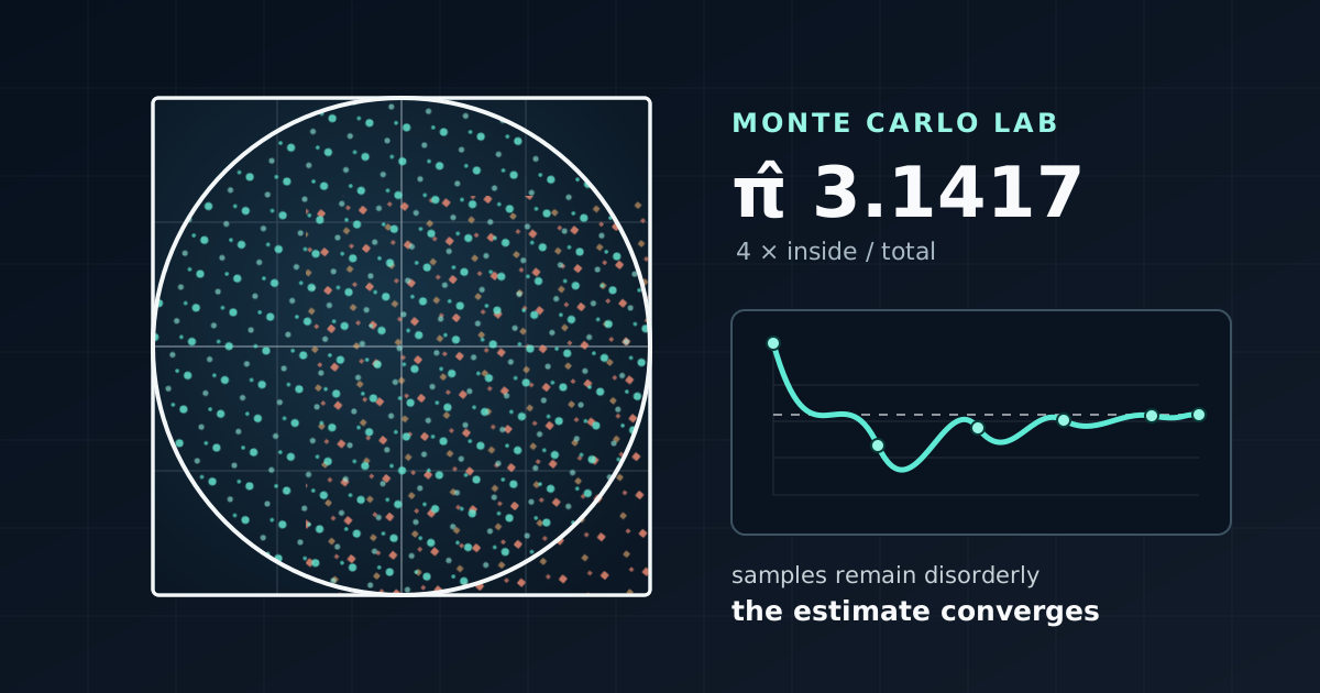
The square represents coordinates from −1 to 1 on both axes. Its circle has radius one. Teal circles mark samples inside; coral diamonds mark samples outside, so the classification does not depend on colour alone. The CPU classifies the numerical coordinates. A custom WebGL2 shader draws only a capped, representative field of those calculated samples; screen resolution cannot change the estimate.

What Monte Carlo means

Monte Carlo is a family of methods, not a single algorithm. Different members of the family simulate particle collisions, financial paths, posterior distributions, molecular configurations, light transport, component failures, and integrals with thousands of dimensions. Their recurring skeleton is simpler than their applications:

1. Describe a domain of possible outcomes and the distribution that belongs on it.
2. Draw samples from that distribution.
3. Evaluate a function, event, or rule at every sample.
4. Average the values or count the events.
5. Quantify how much sampling uncertainty remains.

This fifth step prevents an approximate number from masquerading as a fact. A simulation result without an uncertainty argument may still be useful, but it has left the reader to guess how stable it is.

Estimating π with a square and circle

The square has side length two and area four. The inscribed unit circle has area π. Uniformly chosen points land inside the circle with probability equal to the area ratio:

If N points are drawn and K fall inside, then K/N estimates that probability. Rearranging gives

The little hat means “estimate”. It matters. The calculation does not discover π and, except by coincidence in finite-precision arithmetic, does not produce it exactly. It approximates a deterministic quantity through statistical sampling.

Uniform sampling matters just as much as the counting rule. If points are drawn more frequently near the centre, the circle receives an unfair share and the result estimates the sampler’s bias rather than π. A beautiful animation can therefore be mathematically wrong while looking persuasive. In the live field, classification is the direct test x² + y² ≤ 1, including points exactly on the boundary.

Using the laboratory

Begin with a target of 100 samples. Pause, reset, and press Add 500; the button stops at the selected target. The estimate will probably look unconvincing. Apply a different numerical seed while keeping every other setting fixed. The old samples are explicitly cleared because combining streams from incompatible settings would make the comparison dishonest.

The seed is the starting state of the pseudorandom generator. It makes a run repeatable: same method, seed, target, and sample order; same result. “New random seed” asks the browser for a new 32-bit starting value, but the sequence generated from it is still pseudorandom rather than a measurement of physical randomness.

The sample rate controls how quickly the progressive calculation spends its budget, not which samples are generated. A slow and fast run with identical settings end at the same sequence. Target sample count sets the budget. At 100,000 or one million calculated samples, the instrument may display fewer dots than it has counted. Drawing millions of subpixel marks would waste memory and GPU time without adding information, so the calculated and displayed totals are labelled separately.

Three sampling methods change the sequence itself:

• Pseudorandom uses a seeded Mulberry32 generator to produce independent-looking uniform coordinates. This is the ordinary Monte Carlo baseline.
• Stratified divides the square into cells, visits every cell once per cycle, and jitters a sample inside it. Coverage is deliberately spread out.
• Halton uses a reproducible seed-generated additive shift of radical-inverse sequences in bases two and three. It is a randomized quasi-Monte Carlo construction: deterministic once the seed is fixed, but designed to preserve low-discrepancy coverage.

Use the chart selector to plot the estimate or absolute error. The horizontal axis is logarithmic, and observations are kept only near 10, 20, 50, 100, 200, 500, and so on. This preserves the shape of a long run without storing every animation frame. In pseudorandom error view, the dashed theoretical guide shows one IID standard error with its characteristic 1/√N slope. It is hidden for the other designs because it is not their uncertainty estimate. Every plotted checkpoint is keyboard-focusable and the same data are available in an expandable table.

Why the dots do not become orderly

Convergence is a statement about an aggregate, not a promise that a pseudorandom picture will turn into graph paper. The individual dots remain disorderly. What stabilises is their proportion inside the circle.

The law of large numbers says that, under suitable conditions, the sample proportion approaches the underlying probability as the number of samples grows. It does not say that each new point improves the estimate. A run can move closer to π, wander away, cross it, and wander back. Ten thousand samples may briefly have a larger error than nine thousand. The long-run cloud narrows even though a single path keeps wobbling.

This is why changing the seed at a small budget is instructive. Each seed produces a legitimate run, and their disagreement is visible evidence of sampling variability. Increasing N does not abolish chance; it reduces the scale at which chance disturbs the estimate.

The expensive square-root law

Write p̂ = K/N. For independent Bernoulli classifications, the estimated standard error of the π estimator is

In pseudorandom mode, the instrument uses π̂ ± 1.96 × SE(π̂) as an approximate 95 per cent confidence interval. It appears only after 30 samples because the normal approximation is especially crude at tiny counts. Even later, it is an approximation built on the independent, identically distributed sampling model; it is not a force field guaranteed to contain π in every run.

The denominator contains √N, which creates Monte Carlo’s expensive bargain. Halving the typical error requires roughly four times as many independent samples. Gaining about one extra decimal digit may require around one hundred times as many. These are statistical rates, not promises for each seed, but the log-scaled error chart makes the general slope difficult to miss.

Better sampling, not merely more sampling

Ordinary pseudorandom sampling can leave accidental gaps and clusters. Stratification spends the same budget more evenly: a region that has already supplied its allotted sample cannot consume the entire early run. For the smooth boundary in this two-dimensional example, that often reduces variance.

The shifted Halton sequence goes further. Its underlying points are constructed to keep discrepancy—the mismatch between sampled coverage and ideal uniform coverage—small. A seed-generated additive shift moves the entire sequence reproducibly without turning individual points into IID draws. This randomized quasi-Monte Carlo construction replaces part of random sampling’s clumping with structured space filling.

Neither method is universally superior. Dimensionality, smoothness, discontinuities, coordinate ordering, and correlations all matter. A low-discrepancy sequence can perform poorly when a problem’s important structure is awkwardly aligned, and uncertainty estimation requires a design-aware procedure. For randomized quasi-Monte Carlo, one common approach runs several independent seed shifts and measures variation among their final estimates. Stratification needs variance information from its strata. It also becomes costly when a high-dimensional domain creates an astronomical number of cells. Sampling strategy is part of the model, not a cosmetic dot pattern.

Why anyone uses Monte Carlo

The π problem is almost offensively easy by analytic means. Monte Carlo becomes attractive when direct enumeration or deterministic integration becomes difficult: particle transport through matter, radiation dose modelling, option pricing and financial risk, Bayesian inference, reliability of systems with many failure modes, path-traced rendering, molecular simulation, and uncertainty propagation through complicated models.

Its unusual strength is dimensionality. A good one-dimensional quadrature rule can crush Monte Carlo on a smooth integral. But a problem with hundreds of interacting variables may make a regular grid impossible: ten positions per dimension in one hundred dimensions would require 10 to the power 100 evaluations. Monte Carlo’s basic 1/√N rate is slow, yet that exponent does not directly worsen with dimension. Slow and possible can beat elegant and impossible.

What this demonstration hides

The browser uses finite-precision floating-point numbers. Mulberry32 is a small deterministic generator chosen for reproducibility and teaching, not cryptography. A visually uniform field does not prove independence, and a pattern with clusters is not automatically biased. Confidence intervals rely on a sampling model. The laboratory therefore shows its IID interval only for pseudorandom sampling; stratified and shifted-Halton modes show the same IID expression solely as a labelled reference scale, not as method-specific uncertainty.

The displayed-point cap means a completed million-sample run is not a literal picture of every calculation. The WebGL fragment shader softens point edges and blends density for legibility, but it never votes on whether a point is inside. Context loss can erase a GPU buffer; the CPU state remains the source of truth and is uploaded again if the context returns.

Finally, estimating π is a diagnostic exercise, not a sensible production algorithm. Its known answer lets us detect a biased sampler, a boundary error, or a counting bug. In a real application the answer is unknown, which makes validation harder and the temptation to trust a convincing animation more dangerous.

A closing experiment

Choose a budget of 10,000. Run pseudorandom sampling with several seeds, recording the final error. Repeat with stratification and Halton. Which method usually reaches a small error sooner? Does it win every run? Does error fall smoothly? How large must $N$ become before the first three decimal places look stable?

Then hide the outside points. The estimate does not change because visibility is not evidence. Ask whether the denser-looking field necessarily has the better numerical result. The paradox survives every control: the samples remain uncertain one by one, while carefully measuring them turns uncertainty into a computational tool.