A Skin That Paints Itself

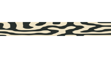
A dark band crosses the first strip from one long edge to the other. In the second strip, charcoal and ivory fold around each other. The outlines match. The first pattern developed inside its strip. The second took shape on a broad patch and was squeezed to fit.

Move Width toward 100%, then bring it back down to 24%. Keep the appearance setting on Stripes and look for a marking that changes direction, joins another marking, or stops short of an edge. Once the new result is ready, Replay formation lets you see when the first strip begins to show its pattern. Then try Tapered patch and follow the markings from the broad end to the tip.

Surface geometry

Does a pattern change when it has less room to form?

Move Width to see what changes. In the first window, the pattern forms inside the new boundary. In the second, a finished pattern is squeezed to fit. The rules and the length stay the same.

A Formed on this shape

B Finished pattern fitted to this shape

Saved example from the model.

Two ways to fill the same strip

At full width the two windows agree. The broad patch and the reference have the same outline, starting disturbance, and rules. Fitting that reference onto a patch of its own size leaves every point where it was. This is a useful check before making the surface narrower. There is no built-in difference in the way the two windows draw the pattern.

On a narrow strip, the first window starts over. At the beginning each point carries nearly the same pair of signal values. The signals interact and spread until the chosen stopping time. They can spread inside the patch, but they do not cross its edges. The boundary is there from the first step of the calculation.

In the other window, each point of the strip looks up a value in the saved broad patch. A point halfway down the strip’s width looks halfway down the width of the reference. Its position along the length stays the same. The lookup blends nearby values where it lands between samples, and then the same pigment rule turns those values into ivory and charcoal. No signals react or spread on that fitted strip. There is only a new place to display the values they reached on the broad patch.

The two windows use the same scale, so narrowing the strip makes it take up less space in both. The cutoff between light and dark also stays put. A value that gives a dark mark in one window gives the same color in the other. Otherwise it would be easy to mistake a change in magnification or contrast for a change in the pattern.

What the signals do

Imagine a place where one signal starts a fraction above its neighbors. The rules allow a small rise to reinforce itself locally. The rise also draws the second signal upward, and that second signal pushes back against the first. The two spread at different rates. The faster one carries the restraint into nearby areas while the initial rise stays fairly local. A peak can hold its ground while making it harder for another peak to develop close by. Farther away, the same rules can allow a second peak.

That is the idea behind the names activator and inhibitor. Both signals are signed numbers, so a value below zero is an ordinary part of the calculation. The pattern view assigns colors from the activator’s value. In the signal views, both windows use a fixed scale with zero marked. Switch views after a run and notice that the shapes and stopping times stay put. The display has changed while the calculation’s result stays the same.

The starting variations are small enough that the beginning of a replay can look blank. Give it a little time. Some variations fade and others build on one another until larger shapes become visible. During replay, the first window shows its current model time. The fitted reference stays at the final time throughout. That lets you watch the markings develop with the finished broad pattern still available for comparison.

The stopping time is a convention. It gives the two calculations an equal chance to develop before we compare them. Model time advances in the calculation’s own units. A run ending at 60 tells us how the fields look at that moment in the model. It gives no timing for a coat on a developing animal.

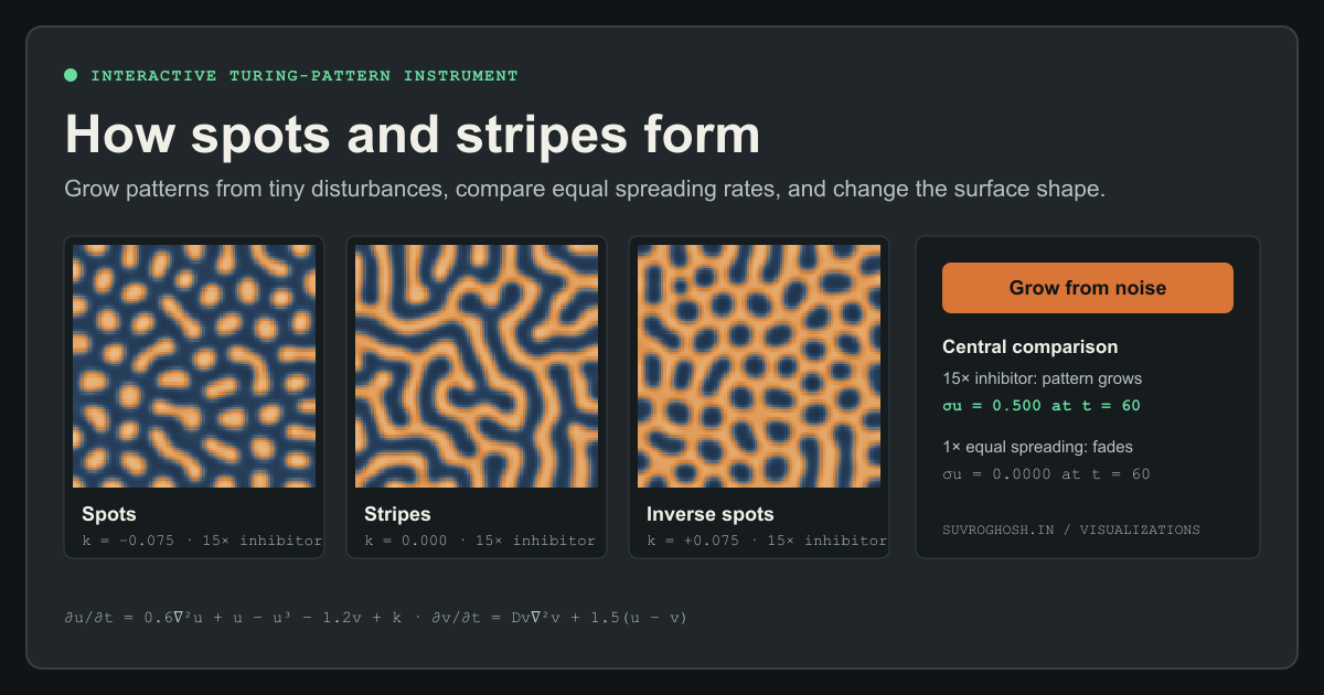
In 1952 Alan Turing showed how reacting and spreading substances could develop a spatial pattern from a nearly uniform state. A small disturbance could grow under the right conditions, with no need to specify in advance where every peak should go. The earlier How spots and stripes form experiment takes up that question directly. It lets you give the signals equal spreading rates and watch the disturbances die down. Here the spreading rates stay fixed and the space available to the signals changes.

What gets harder to fit

A variation can run along a patch, across it, or in both directions. In a broad rectangle there is room for a marking to bend around another one and for several changes from high to low signal across the width. A narrow rectangle still leaves the same distance from one end to the other, but the two long edges are closer together. The same spreading distances now take up a larger fraction of the width. A variation that could develop across the broad patch may fare poorly across the strip, while one that runs along its length can still develop.

One way to picture the constraint is to imagine a row of highs and lows across the width. Squeeze the row and each high gets closer to the next low. Diffusion smooths out changes over short distances especially quickly. In the forming panel, a variation that would need those short distances may fade before it makes a visible mark. In the fitted panel, the row can be squeezed after the signals have stopped. That is how a thin set of markings can survive in one view even where there is no matching set in the other.

The edge matters even though no signal flows through it. At an interior point the signal can spread into adjacent parts of the surface on either side. At the boundary some of that neighboring surface is missing. The model accounts for that by giving the missing neighbor zero exchange with the point at the edge. In the continuous description, the signal’s slope in the direction out of the patch is zero at the wall. It can still vary along the wall.

Starting disturbances matter too. If one strip had a completely different random start from another, a different-looking pattern would tell us less about the role of the boundary. Here the seed is used to give the same prescribed disturbance to a point at the same physical coordinates. The wide patch has additional points outside the strip. Where the two patches overlap, they agree at the start. Replay lets you watch how they can come to disagree.

From a broad patch to a narrow strip

The worked example uses Stripes, starting disturbance 1952, and a stopping time of 60 in model time. The full rectangle is 76.8 units long and 40 units wide. The strip keeps the length and uses 9.6 units of width, or 24% of the original. The two signals still spread at the same respective rates and interact by the same rules. The spacing between neighboring sample points and the time step also stay fixed.

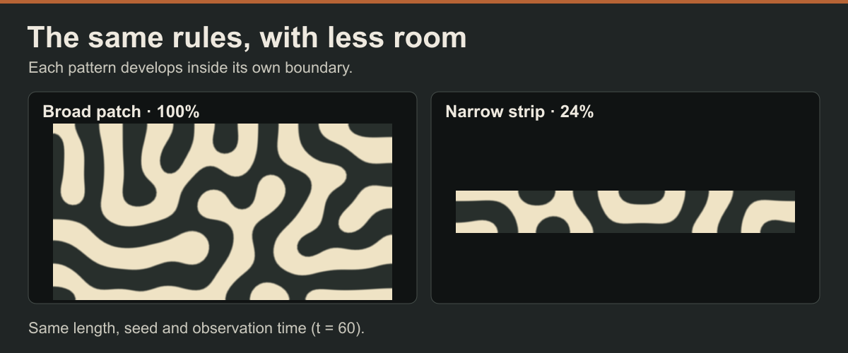
Look about four-fifths of the way from the left end. In the pattern formed inside the strip, a dark band reaches both long edges. The fitted pattern still divides the width into light and dark there. It can put several folds of the old pattern across a very small width because those folds took shape when there was more room. A different seed can shift where particular markings land. This example shows that changing the width can change the arrangement. Where any one stripe lands depends on the run.

One patch that narrows

The taper brings the wide and narrow parts into one calculation. The preset starts 32 units wide at the left and narrows toward 8 at the right. In the fitted panel, the amount of squeeze depends on where you are along the length. At the broad end there is less compression. Toward the tip, the same span of the reference goes into a much smaller width. In the first window every part of the patch is in contact with its neighbors as the pattern develops.

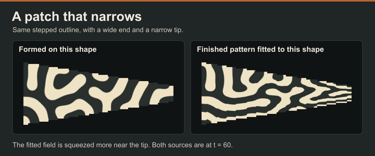
Follow the stripes in the formed panel. At the broad end several branches share the width. Near the narrow end a band crosses it. Beside it, the fitted panel squeezes the branches already present in the broad rectangle. A taper drawn on a square grid has a stepped edge, and both windows share that outline. The tip still has several cells across it at the smallest supported setting. A band crossing it is a marking on a flat patch. Calling it a ring would require a surface that wraps around.

The biological question

James D. Murray treats reaction and diffusion in the first volume of his third edition of Mathematical Biology. The second volume develops spatial pattern formation, considers animal coats, and then turns to patterns on growing domains. The geometry question matters there because a developmental process runs in a body with a particular shape and size. Seeing a marking on the finished body only tells us where it ended up. The available space while it formed may have been quite different.

The two signals here belong to an illustrative cubic model. Their values give a way to ask a controlled question about boundaries. An animal coat involves tissue, cells, and mechanisms that produce pigment. Evidence about those mechanisms would have to come from the animal and its development. A resemblance between one of these pictures and a coat marking can suggest a question for that investigation.

Changing the width starts a new calculation on the selected surface. During that calculation the surface stays fixed. In growing tissue the boundary can move while the signals are changing, and the tissue can carry the signals along and spread them over more area. A model of that process would need to say where and how quickly the tissue grows and what happens to each signal as it moves. Squeezing a finished field gives us a comparison to look at, while a growth model would have to account for changes throughout formation.

Return to Narrow strip and look just to the right of center. A dark inlet in the formed strip stops short of the bottom edge. Follow the strip a little farther to the right and the next dark band reaches it. In the fitted strip, a thin ivory line follows that part of the bottom edge.

P.S. References

• Alan M. Turing, The Chemical Basis of Morphogenesis (1952), the original paper on how a nearly uniform system can develop a spatial pattern. Original paper, hosted by MIT
• J. D. Murray, Mathematical Biology I. An Introduction, 3rd ed. (Springer, 2002), chapter 11 for the introduction to reaction and diffusion. Springer
• J. D. Murray, Mathematical Biology II. Spatial Models and Biomedical Applications, 3rd ed. (Springer, 2003), chapters 2–4 on spatial patterns, animal coats, and growing domains. Springer